Extended Two-Way Fixed Effects (ETWFE)#
There is nothing wrong with TWFE for staggered DiD as long as the model is flexible enough. The Extended TWFE approach adds cohort-by-time interaction dummies so that each (cohort, period) cell gets its own treatment effect coefficient. The estimates are numerically identical to a cohort imputation procedure and to random effects. The issue with conventional TWFE was never the estimator; it was the constant-effect specification that forced all those heterogeneous effects into one number.
See also
Extended TWFE background for the equivalence proofs and nonlinear extensions, and Staggered DiD for the Callaway and Sant’Anna estimator applied to the same data.
Empirical application#
This example studies the effect of minimum wage increases on teen employment, using the same Quarterly Workforce Indicators data as the Staggered DiD example.
From 2001 to 2007, the US federal minimum wage was flat at $5.15 per hour. Some states raised their minimum wage above the federal level during this period while others did not. The variation in timing creates a staggered adoption design with treatment cohorts in 2004, 2006, and 2007. States that kept the federal minimum serve as a never-treated control group.
The outcome is log county-level teen employment. The dataset contains 500 counties observed annually from 2003 to 2007. The hypothesis is that minimum wage increases reduce teen employment, since teenagers are disproportionately represented among minimum wage workers.
ETWFE is well-suited to this setting because it handles the staggered rollout through a single regression with cohort-by-time interactions, rather than the semiparametric approach of Callaway and Sant’Anna. It also extends naturally to nonlinear models (Poisson, logit), which is useful when the parallel trends assumption is more plausible on a transformed scale.
Loading the data#
import moderndid as did

data = did.load_mpdta()
print(data.head())
shape: (5, 6)
┌──────┬────────────┬──────────┬──────────┬─────────────┬───────┐
│ year ┆ countyreal ┆ lpop     ┆ lemp     ┆ first.treat ┆ treat │
│ ---  ┆ ---        ┆ ---      ┆ ---      ┆ ---         ┆ ---   │
│ i64  ┆ i64        ┆ f64      ┆ f64      ┆ i64         ┆ i64   │
╞══════╪════════════╪══════════╪══════════╪═════════════╪═══════╡
│ 2003 ┆ 8001       ┆ 5.896761 ┆ 8.461469 ┆ 2007        ┆ 1     │
│ 2004 ┆ 8001       ┆ 5.896761 ┆ 8.33687  ┆ 2007        ┆ 1     │
│ 2005 ┆ 8001       ┆ 5.896761 ┆ 8.340217 ┆ 2007        ┆ 1     │
│ 2006 ┆ 8001       ┆ 5.896761 ┆ 8.378161 ┆ 2007        ┆ 1     │
│ 2007 ┆ 8001       ┆ 5.896761 ┆ 8.487352 ┆ 2007        ┆ 1     │
└──────┴────────────┴──────────┴──────────┴─────────────┴───────┘
The dataset contains 500 counties observed from 2003 to 2007. Treatment
cohorts are 2004, 2006, and 2007, with first.treat = 0 for counties that
never raised their minimum wage. The outcome lemp is log teen employment.
Estimation#
etwfe estimates a saturated regression with cohort-by-time
interactions and absorbed unit and time fixed effects. The interface mirrors
att_gt with the same core arguments.
mod = did.etwfe(
    data=data,
    yname="lemp",
    tname="year",
    gname="first.treat",
    idname="countyreal",
)
print(mod)
==============================================================================
 Extended Two-Way Fixed Effects (ETWFE)
==============================================================================

┌───────┬──────┬──────────┬────────────┬────────────────────────────┐
│ Group │ Time │ ATT(g,t) │ Std. Error │ [95% Pointwise Conf. Band] │
├───────┼──────┼──────────┼────────────┼────────────────────────────┤
│  2004 │ 2004 │  -0.0194 │     0.0308 │ [-0.0798,  0.0410]         │
│  2004 │ 2005 │  -0.0783 │     0.0276 │ [-0.1323, -0.0243] *       │
│  2004 │ 2006 │  -0.1361 │     0.0304 │ [-0.1957, -0.0765] *       │
│  2006 │ 2006 │   0.0025 │     0.0181 │ [-0.0331,  0.0381]         │
│  2004 │ 2007 │  -0.1047 │     0.0329 │ [-0.1693, -0.0401] *       │
│  2006 │ 2007 │  -0.0392 │     0.0217 │ [-0.0816,  0.0033]         │
│  2007 │ 2007 │  -0.0431 │     0.0179 │ [-0.0782, -0.0080] *       │
└───────┴──────┴──────────┴────────────┴────────────────────────────┘

------------------------------------------------------------------------------
 Signif. codes: '*' confidence band does not cover 0

------------------------------------------------------------------------------
 Data Info
------------------------------------------------------------------------------
 Control Group:  Not Yet Treated
 Observations:  2500
 Units:  500
 Fixed Effects:  countyreal + year

------------------------------------------------------------------------------
 Estimation Details
------------------------------------------------------------------------------
 Estimation Method:  Extended TWFE (OLS)
 R-squared:  0.9933

------------------------------------------------------------------------------
 Inference
------------------------------------------------------------------------------
 Significance level: 0.05
 Std. errors: hetero
==============================================================================
 Reference: Wooldridge (2021, 2023)
Each row is a cohort-time ATT, the average effect for units first treated in
the Group year, measured at the Time year. The default control group is
"notyet" (not-yet-treated units), which is why the table only includes
post-treatment cells. The 2004 cohort shows growing effects from -0.02 at
impact to -0.14 two years later, consistent with a lagged employment response.
The 2007 cohort has a single post-treatment period with an effect of -0.04.
Aggregating treatment effects#
With seven cohort-time estimates there is a lot to take in.
emfx aggregates them into simpler summaries, playing the
same role that aggte plays for the Callaway and Sant’Anna
estimator.
Overall effect#
simple = did.emfx(mod, type="simple")
print(simple)
==============================================================================
 Aggregate Treatment Effects (Simple Average)
==============================================================================

 Overall ATT:

┌─────────┬────────────┬────────────────────────┐
│     ATT │ Std. Error │ [95% Conf. Interval]   │
├─────────┼────────────┼────────────────────────┤
│ -0.0477 │     0.0123 │ [ -0.0719,  -0.0235] * │
└─────────┴────────────┴────────────────────────┘

------------------------------------------------------------------------------
 Signif. codes: '*' confidence band does not cover 0

------------------------------------------------------------------------------
 Data Info
------------------------------------------------------------------------------
 Control Group:  Not Yet Treated
 Observations:  2500
 Units:  500

------------------------------------------------------------------------------
 Estimation Details
------------------------------------------------------------------------------
 Estimation Method:  Extended TWFE (OLS)

------------------------------------------------------------------------------
 Inference
------------------------------------------------------------------------------
 Significance level: 0.05
 Delta method standard errors
==============================================================================
 Reference: Wooldridge (2021, 2023)
The overall ATT of -0.048 means minimum wage increases reduced log teen employment by about 4.8 percent on average across all treated counties and post-treatment periods. For comparison, Callaway and Sant’Anna give an overall ATT of -0.040 on the same data (see the Staggered DiD example). The gap is small and stems from the different default control groups (not-yet-treated vs never-treated) and from differences in how the two methods handle weighting.
Event study#
To get both pre-treatment and post-treatment event times, we re-estimate with
cgroup="never". With a never-treated control group, the treatment
indicator preserves pre-treatment variation and the event study includes
negative event times that serve as a placebo test for parallel trends.
mod_never = did.etwfe(
    data=data,
    yname="lemp",
    tname="year",
    gname="first.treat",
    idname="countyreal",
    cgroup="never",
)
event = did.emfx(mod_never, type="event", window=(-3, 3))
print(event)
==============================================================================
 Aggregate Treatment Effects (Event Study)
==============================================================================

 Overall summary of ATT's based on event-study/dynamic aggregation:

┌─────────┬────────────┬────────────────────────┐
│     ATT │ Std. Error │ [95% Conf. Interval]   │
├─────────┼────────────┼────────────────────────┤
│ -0.0050 │     0.0111 │ [ -0.0267,   0.0167]   │
└─────────┴────────────┴────────────────────────┘


 Dynamic Effects:

┌────────────┬──────────┬────────────┬────────────────────────────┐
│ Event time │ Estimate │ Std. Error │ [95% Pointwise Conf. Band] │
├────────────┼──────────┼────────────┼────────────────────────────┤
│         -3 │   0.0250 │     0.0161 │ [-0.0066,  0.0567]         │
│         -2 │   0.0245 │     0.0144 │ [-0.0038,  0.0527]         │
│          0 │  -0.0199 │     0.0152 │ [-0.0498,  0.0099]         │
│          1 │  -0.0510 │     0.0177 │ [-0.0857, -0.0162] *       │
│          2 │  -0.1373 │     0.0315 │ [-0.1989, -0.0756] *       │
│          3 │  -0.1008 │     0.0334 │ [-0.1663, -0.0353] *       │
└────────────┴──────────┴────────────┴────────────────────────────┘

------------------------------------------------------------------------------
 Signif. codes: '*' confidence band does not cover 0

------------------------------------------------------------------------------
 Data Info
------------------------------------------------------------------------------
 Control Group:  Never Treated
 Observations:  2500
 Units:  500

------------------------------------------------------------------------------
 Estimation Details
------------------------------------------------------------------------------
 Estimation Method:  Extended TWFE (OLS)

------------------------------------------------------------------------------
 Inference
------------------------------------------------------------------------------
 Significance level: 0.05
 Delta method standard errors
==============================================================================
 Reference: Wooldridge (2021, 2023)
The window=(-3, 3) argument trims the event times to match the range
available from the Callaway and Sant’Anna estimator, making comparison
straightforward. Event time -1 is the excluded reference period for each
cohort and does not appear. The pre-treatment estimates at event times -3
and -2 are small and insignificant, consistent with parallel trends. The
post-treatment effects grow from -0.02 at impact to -0.14 after two years
before moderating to -0.10 at event time 3.
With the default cgroup="notyet", pre-treatment effects are
mechanistically zero because the not-yet-treated reference group absorbs all
pre-treatment variation. Switching to cgroup="never" is what gives us
actual pre-treatment estimates for diagnostics.
Group effects#
by_group = did.emfx(mod, type="group")
print(by_group)
==============================================================================
 Aggregate Treatment Effects (Group/Cohort)
==============================================================================

 Overall summary of ATT's based on group/cohort aggregation:

┌─────────┬────────────┬────────────────────────┐
│     ATT │ Std. Error │ [95% Conf. Interval]   │
├─────────┼────────────┼────────────────────────┤
│ -0.0477 │     0.0123 │ [ -0.0719,  -0.0235] * │
└─────────┴────────────┴────────────────────────┘


 Group Effects:

┌───────┬──────────┬────────────┬────────────────────────────┐
│ Group │ Estimate │ Std. Error │ [95% Pointwise Conf. Band] │
├───────┼──────────┼────────────┼────────────────────────────┤
│  2004 │  -0.0846 │     0.0250 │ [-0.1336, -0.0356] *       │
│  2006 │  -0.0183 │     0.0160 │ [-0.0496,  0.0129]         │
│  2007 │  -0.0431 │     0.0179 │ [-0.0782, -0.0080] *       │
└───────┴──────────┴────────────┴────────────────────────────┘

------------------------------------------------------------------------------
 Signif. codes: '*' confidence band does not cover 0

------------------------------------------------------------------------------
 Data Info
------------------------------------------------------------------------------
 Control Group:  Not Yet Treated
 Observations:  2500
 Units:  500

------------------------------------------------------------------------------
 Estimation Details
------------------------------------------------------------------------------
 Estimation Method:  Extended TWFE (OLS)

------------------------------------------------------------------------------
 Inference
------------------------------------------------------------------------------
 Significance level: 0.05
 Delta method standard errors
==============================================================================
 Reference: Wooldridge (2021, 2023)
Early adopters (2004 cohort) experienced the largest effect at -0.08, while the 2006 cohort shows a smaller, insignificant effect of -0.02. This heterogeneity is consistent with the Callaway and Sant’Anna group estimates of -0.08, -0.02, and -0.03 for the same cohorts.
Plotting the event study#
from plotnine import labs, theme, theme_gray

p = did.plot_event_study(event, ref_period=-1)
p = (p
    + labs(
        x="Years Relative to Treatment",
        y="ATT (Log Employment)",
        title="ETWFE Event Study",
        subtitle="Dynamic treatment effects with never-treated controls",
    )
    + theme_gray()
    + theme(legend_position="bottom")
)
p.save("plot_etwfe_event_study.png", dpi=200, width=8, height=5)
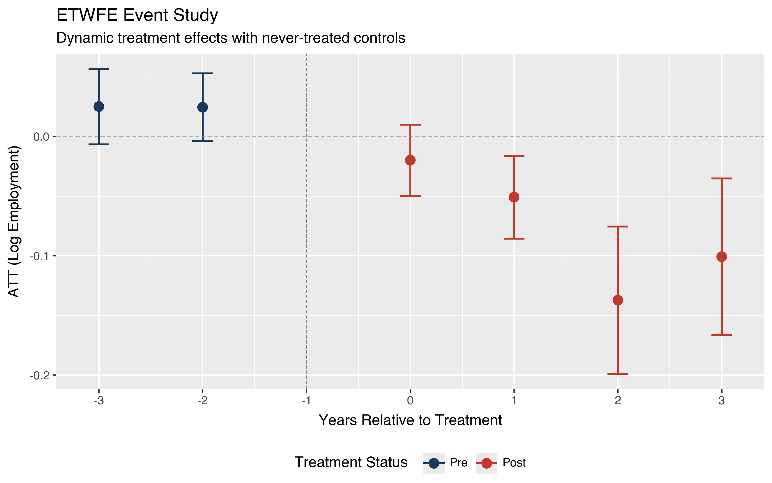
The pre-treatment estimates are flat and close to zero. The post-treatment effects grow with exposure time and are all statistically significant from event time 1 onward.
Comparing ETWFE and Callaway-Sant’Anna#
Both estimators target the same cohort-time ATTs but arrive at them through different identification strategies. For an apples-to-apples comparison we run both with never-treated controls so that both produce pre-treatment event times.
from plotnine import (
    aes, geom_errorbar, geom_hline, geom_point, geom_vline,
    ggplot, labs, position_dodge, scale_color_manual,
    scale_shape_manual, scale_x_continuous, theme, theme_gray,
)
# CS with never-treated controls
result_cs = did.att_gt(
    data=data, yname="lemp", tname="year",
    gname="first.treat", idname="countyreal", boot=False,
)
event_cs = did.aggte(result_cs, type="dynamic")
# Combine (event already uses window=(-3, 3) from above)
import polars as pl

etwfe_df = did.to_df(event).with_columns(pl.lit("ETWFE").alias("estimator"))
cs_df = did.to_df(event_cs).with_columns(pl.lit("CS").alias("estimator"))
plot_df = pl.concat([etwfe_df, cs_df])
dodge = position_dodge(width=0.3)

p = (
    ggplot(plot_df, aes(x="event_time", y="att",
                        color="estimator", shape="estimator"))
    + geom_hline(yintercept=0, color="black", size=0.4)
    + geom_vline(xintercept=-0.5, linetype="dashed",
                 color="gray", size=0.4)
    + geom_errorbar(
        aes(ymin="ci_lower", ymax="ci_upper"),
        width=0.15, size=0.6, position=dodge,
    )
    + geom_point(size=3, position=dodge)
    + scale_color_manual(
        values={"ETWFE": "#c0392b", "CS": "#1a3a5c"})
    + scale_shape_manual(
        values={"ETWFE": "^", "CS": "o"})
    + scale_x_continuous(
        breaks=sorted(
            set(plot_df["event_time"].unique().to_list()) | {-1}),
    )
    + labs(
        x="Years Relative to Treatment",
        y="ATT (Log Employment)",
        title="Comparing ETWFE and Callaway-Sant'Anna"
              " Event Studies",
        subtitle="Both estimators use never-treated controls",
        color="", shape="",
    )
    + theme_gray()
    + theme(legend_position="right")
)
p.save("plot_etwfe_vs_cs.png", dpi=200, width=8, height=5)
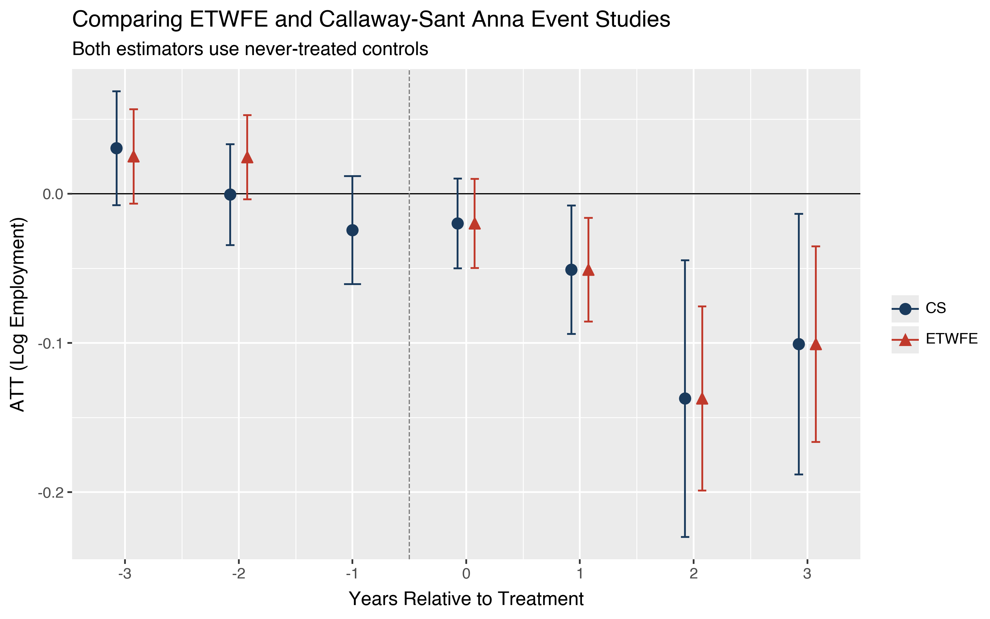
Both estimators show pre-treatment and post-treatment event times. The post-treatment estimates (event times 0 through 3) are nearly identical, which is expected since both use the same never-treated control group. The pre-treatment estimates differ slightly because the two methods use different reference periods and handle the pre-treatment comparisons differently, but both are small and close to zero, consistent with parallel trends.
ETWFE (Wooldridge) |
CS (Callaway-Sant’Anna) |
|
|---|---|---|
Identification |
Saturated regression with cohort-time interactions |
Semiparametric (IPW, OR, or doubly robust) |
Default control group |
Not-yet-treated |
Never-treated |
Pre-trends test |
Set |
Built-in via pre-treatment ATTs |
Covariates |
Demeaned within cohorts (Mundlak device) |
Propensity score and/or outcome regression |
Nonlinear models |
Poisson, logit, probit via |
Not available |
Inference |
Heteroskedasticity-robust or cluster-robust |
Analytical or multiplier bootstrap |
On this dataset the two methods tell a similar story. Seeing consistent results from a regression-based approach and a semiparametric approach on the same data is a good sign. Divergence between the two would warrant a closer look at which identifying assumptions are more credible.
Adding covariates#
Time-constant covariates can be added through xformla. The estimator
automatically demeans them within cohort groups so that the parallel trends
assumption need only hold conditional on the covariates.
mod_cov = did.etwfe(
    data=data,
    yname="lemp",
    tname="year",
    gname="first.treat",
    idname="countyreal",
    xformla="~lpop",
)
print(did.emfx(mod_cov, type="simple"))
Adding log population as a control changes the estimates slightly, since it allows for different employment trends across counties of different sizes.
Choosing the control group#
By default, ETWFE uses not-yet-treated units as controls (cgroup="notyet").
This drops observations once the reference cohort enters treatment. To use
only never-treated units, set cgroup="never". As shown above, the
never-treated option also enables pre-treatment event times for diagnostics.
mod_never = did.etwfe(
    data=data,
    yname="lemp",
    tname="year",
    gname="first.treat",
    idname="countyreal",
    cgroup="never",
)
print(did.emfx(mod_never, type="simple"))
The never-treated control group is more restrictive (requires a sufficient number of never-treated units) but avoids the concern that future treatment may contaminate the control group.
Variance-covariance options#
Standard errors default to heteroskedasticity-robust ("hetero"). To
cluster at a specific level, pass a dictionary to vcov.
mod_cluster = did.etwfe(
    data=data,
    yname="lemp",
    tname="year",
    gname="first.treat",
    idname="countyreal",
    vcov={"CRV1": "first.treat"},
)
print(did.emfx(mod_cluster, type="simple"))
Clustering by first.treat accounts for within-cohort correlation. In
practice, you should cluster at the level of treatment assignment.
Nonlinear models#
When the outcome is binary, fractional, or a count, the standard linear
parallel trends assumption may be unrealistic. The family argument
switches to a nonlinear model that imposes parallel trends on the index
scale instead.
mod_pois = did.etwfe(
    data=data,
    yname="lemp",
    tname="year",
    gname="first.treat",
    family="poisson",
)
print(did.emfx(mod_pois, type="simple"))
==============================================================================
 Aggregate Treatment Effects (Simple Average)
==============================================================================

 Overall ATT:

┌─────────┬────────────┬────────────────────────┐
│     ATT │ Std. Error │ [95% Conf. Interval]   │
├─────────┼────────────┼────────────────────────┤
│ -0.0492 │     0.1503 │ [ -0.3439,   0.2455]   │
└─────────┴────────────┴────────────────────────┘

------------------------------------------------------------------------------
 Signif. codes: '*' confidence band does not cover 0

------------------------------------------------------------------------------
 Data Info
------------------------------------------------------------------------------
 Control Group:  Not Yet Treated
 Observations:  2500
 Units:  2500

------------------------------------------------------------------------------
 Estimation Details
------------------------------------------------------------------------------
 Estimation Method:  Extended TWFE (poisson)

------------------------------------------------------------------------------
 Inference
------------------------------------------------------------------------------
 Significance level: 0.05
 Delta method standard errors
==============================================================================
 Reference: Wooldridge (2021, 2023)
The Poisson overall ATT of -0.049 is on the response scale, obtained by differencing counterfactual predictions through the exponential inverse link function. The effect is smaller in magnitude and not statistically significant, reflecting the different identifying assumption (parallel trends in growth rates rather than in levels).
Poisson QMLE with an exponential mean function assumes parallel trends in
growth rates rather than in levels. This is often more plausible for
nonnegative outcomes. "logit" and "probit" are also available for
binary and fractional outcomes.
For non-Gaussian families, unit fixed effects cannot be absorbed (due to the
incidental parameters problem), so fe is automatically set to "none"
and idname is ignored. The estimation uses cohort dummies instead.
The marginal effects from emfx are computed on the
response scale by differencing counterfactual predictions through the inverse
link function, with delta-method standard errors.
GPU acceleration#
For large datasets, the backend argument passes through to pyfixest’s
demeaner, enabling GPU-accelerated fixed-effects absorption via CuPy.
mod_gpu = did.etwfe(
    data=data,
    yname="lemp",
    tname="year",
    gname="first.treat",
    idname="countyreal",
    backend="cupy",
)
This requires CuPy and a CUDA-capable GPU. Without a GPU, pyfixest silently
falls back to a CPU solver. "jax" is another GPU-capable option (requires
JAX with GPU support). CPU-only alternatives include "numba" (the default),
"rust", and "scipy". The backend only affects the fixed-effects
demeaning step and does not change the numerical results. See the
pyfixest documentation for details.
Next steps#
For API details and additional options, see the ETWFE API reference.
For theoretical background on the ETWFE methodology, including the imputation equivalence and nonlinear extensions, see the Extended TWFE background.
For sensitivity analysis of the parallel trends assumption, see the Honest DiD walkthrough.