
Nonparametric Instrumental Variables Estimation#
Parametric IV commits to a functional form before seeing the data. If the true relationship is nonlinear in a way the specification misses, the estimates will be wrong across the entire support, not just at the extremes. The Chen, Christensen, and Kankanala (2024) estimator lets the data determine the shape by approximating the unknown function with B-spline sieves whose complexity is chosen adaptively. The output is a curve with uniform confidence bands rather than a table of pointwise intervals.
Within ModernDiD, this estimator also serves as the engine behind the
nonparametric (CCK) dose-response estimator in cont_did
(see Continuous DiD).
See also
Nonparametric Instrumental Variables for the sieve TSLS framework, data-driven dimension selection, and minimax rate results.
Empirical application#
The relationship between household spending on food and total income has been studied since Ernst Engel first observed in 1857 that poorer households devote a larger share of their budget to food. This negative relationship, known as Engel’s law, is one of the best-established empirical regularities in economics.
Estimating the Engel curve flexibly is complicated by the endogeneity of total expenditure. Households that enjoy food more tend to both spend more in total and allocate a larger share to food, biasing a naive regression. Instrumental variables solve this by using a variable that shifts total expenditure but does not directly affect food preferences. Wages are a natural candidate, since they determine purchasing power but are plausibly excluded from the food share equation once we condition on total spending.
We use the 1995 British Family Expenditure Survey, which contains expenditure shares and income measures for 1,655 households (married or cohabiting couples with an employed head of household aged 25 to 55 with at most two children). The challenge is that we do not want to assume a particular functional form for the relationship. NPIV lets us estimate the curve flexibly while correcting for the endogeneity of expenditure.
Loading the data#
The Engel dataset from the 1995 British Family Expenditure Survey contains the three variables we need.
import numpy as np
import polars as pl
import moderndid as did

df = did.load_engel()
print(df.select("food", "logexp", "logwages").head(10))
shape: (10, 3)
┌──────────┬──────────┬──────────┐
│ food     ┆ logexp   ┆ logwages │
│ ---      ┆ ---      ┆ ---      │
│ f64      ┆ f64      ┆ f64      │
╞══════════╪══════════╪══════════╡
│ 0.28026  ┆ 3.609024 ┆ 5.013565 │
│ 0.379358 ┆ 3.933002 ┆ 2.71866  │
│ 0.226277 ┆ 4.064315 ┆ 3.881564 │
│ 0.167698 ┆ 4.130275 ┆ 4.900374 │
│ 0.343115 ┆ 4.259548 ┆ 5.564099 │
│ 0.132538 ┆ 4.27743  ┆ 5.105824 │
│ 0.626101 ┆ 4.293947 ┆ 5.819371 │
│ 0.245819 ┆ 4.297966 ┆ 5.521221 │
│ 0.478148 ┆ 4.34374  ┆ 4.697293 │
│ 0.453383 ┆ 4.359142 ┆ 5.702281 │
└──────────┴──────────┴──────────┘
Three columns matter here. food is the food expenditure share (our
outcome). logexp is log total expenditure (our potentially endogenous
regressor). logwages is log wages (our instrument). The economic logic is
that wages shift total expenditure but are plausibly excluded from the food
share equation once we condition on total spending.
Estimating the Engel curve#
We estimate the nonparametric Engel curve by instrumenting food share on log-expenditure with log-wages. To visualize the curve, we evaluate the estimate on a uniform grid of 100 points over the range of log-expenditure, which makes for cleaner plots.
logexp_eval = np.linspace(4.5, 6.5, 100).reshape(-1, 1)

result = did.npiv(
    data=df,
    yname="food",
    xname="logexp",
    wname="logwages",
    x_eval=logexp_eval,
    j_x_segments=5,
    biters=200,
    seed=42,
)
print(f"Estimates at {len(result.h)} grid points")
print(f"95% UCB critical value: {result.cv:.3f}")
print(f"Basis: degree={result.j_x_degree}, segments={result.j_x_segments}")
Estimates at 100 grid points
95% UCB critical value: 2.811
Basis: degree=3, segments=5
The result is an NPIVResult containing the estimated
function h, 95% uniform confidence bands h_lower and h_upper,
derivative estimates deriv, pointwise standard errors asy_se, and
bootstrap critical values cv and cv_deriv.
Plotting the estimated curve#
The estimated Engel curve shows how food share varies with total expenditure. The solid line is the IV estimate, the dashed lines are the 95% uniform confidence bands, and the shaded region highlights the area between them.
from plotnine import ggplot, aes, geom_line, geom_ribbon, labs, theme_gray, theme, element_text

plot_df = pl.DataFrame({
    "logexp": logexp_eval.ravel(),
    "Estimate": result.h,
    "Lower": result.h_lower,
    "Upper": result.h_upper,
}).to_pandas()

p = (
    ggplot(plot_df, aes(x="logexp"))
    + geom_ribbon(aes(ymin="Lower", ymax="Upper"), alpha=0.2, fill="#5b7ea4")
    + geom_line(aes(y="Upper"), linetype="dashed", color="#2c3e50", size=0.5)
    + geom_line(aes(y="Lower"), linetype="dashed", color="#2c3e50", size=0.5)
    + geom_line(aes(y="Estimate"), color="#2c3e50", size=1)
    + labs(
        x="Log Expenditure",
        y="Food Share",
        title="Estimated Engel Curve",
        subtitle="Nonparametric IV estimate with 95% uniform confidence bands",
    )
    + theme_gray()
    + theme(
        plot_title=element_text(size=13, weight="bold"),
        plot_subtitle=element_text(size=10),
    )
)
p.save("plot_npiv_engel.png", dpi=200, width=8, height=5)
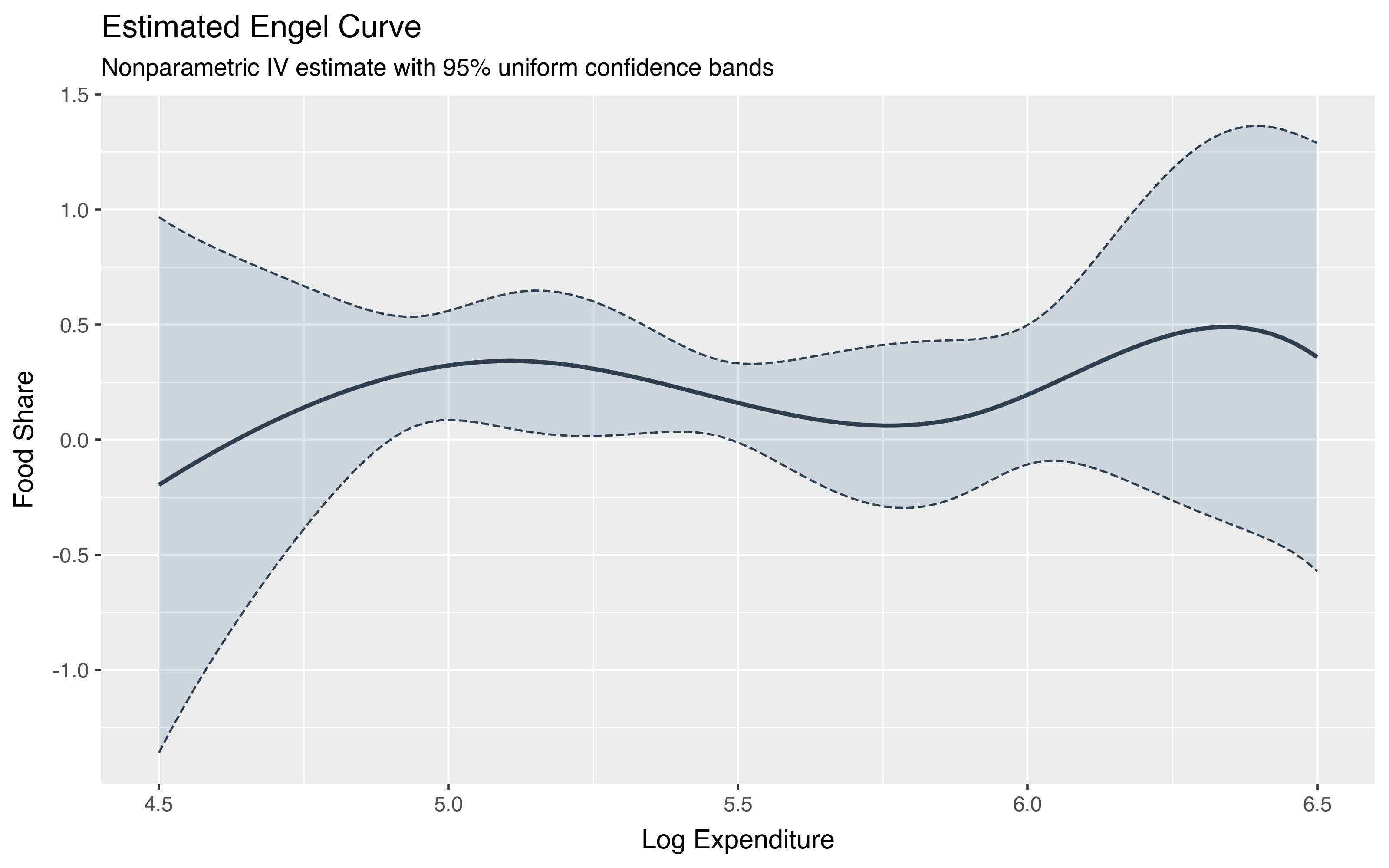
The estimated food share is declining over most of the range, consistent with Engel’s law that food is a necessity. The confidence bands widen near the boundaries of the support where fewer observations are available and narrow in the interior where the estimate is more precise.
Derivative estimation#
The derivative of the Engel curve is the marginal propensity to spend on food
as total expenditure changes. In a nonparametric model, this is the slope of
the structural function at each point. The npiv function
estimates derivatives and their uniform confidence bands simultaneously with
the function estimate.
deriv_df = pl.DataFrame({
    "logexp": logexp_eval.ravel(),
    "Estimate": result.deriv,
    "Lower": result.h_lower_deriv,
    "Upper": result.h_upper_deriv,
}).to_pandas()

p = (
    ggplot(deriv_df, aes(x="logexp"))
    + geom_ribbon(aes(ymin="Lower", ymax="Upper"), alpha=0.2, fill="#5b7ea4")
    + geom_line(aes(y="Upper"), linetype="dashed", color="#2c3e50", size=0.5)
    + geom_line(aes(y="Lower"), linetype="dashed", color="#2c3e50", size=0.5)
    + geom_line(aes(y="Estimate"), color="#2c3e50", size=1)
    + labs(
        x="Log Expenditure",
        y="Derivative of Food Share",
        title="Engel Curve Derivative",
        subtitle="Marginal propensity to spend on food with 95% uniform confidence bands",
    )
    + theme_gray()
    + theme(
        plot_title=element_text(size=13, weight="bold"),
        plot_subtitle=element_text(size=10),
    )
)
p.save("plot_npiv_deriv.png", dpi=200, width=8, height=5)
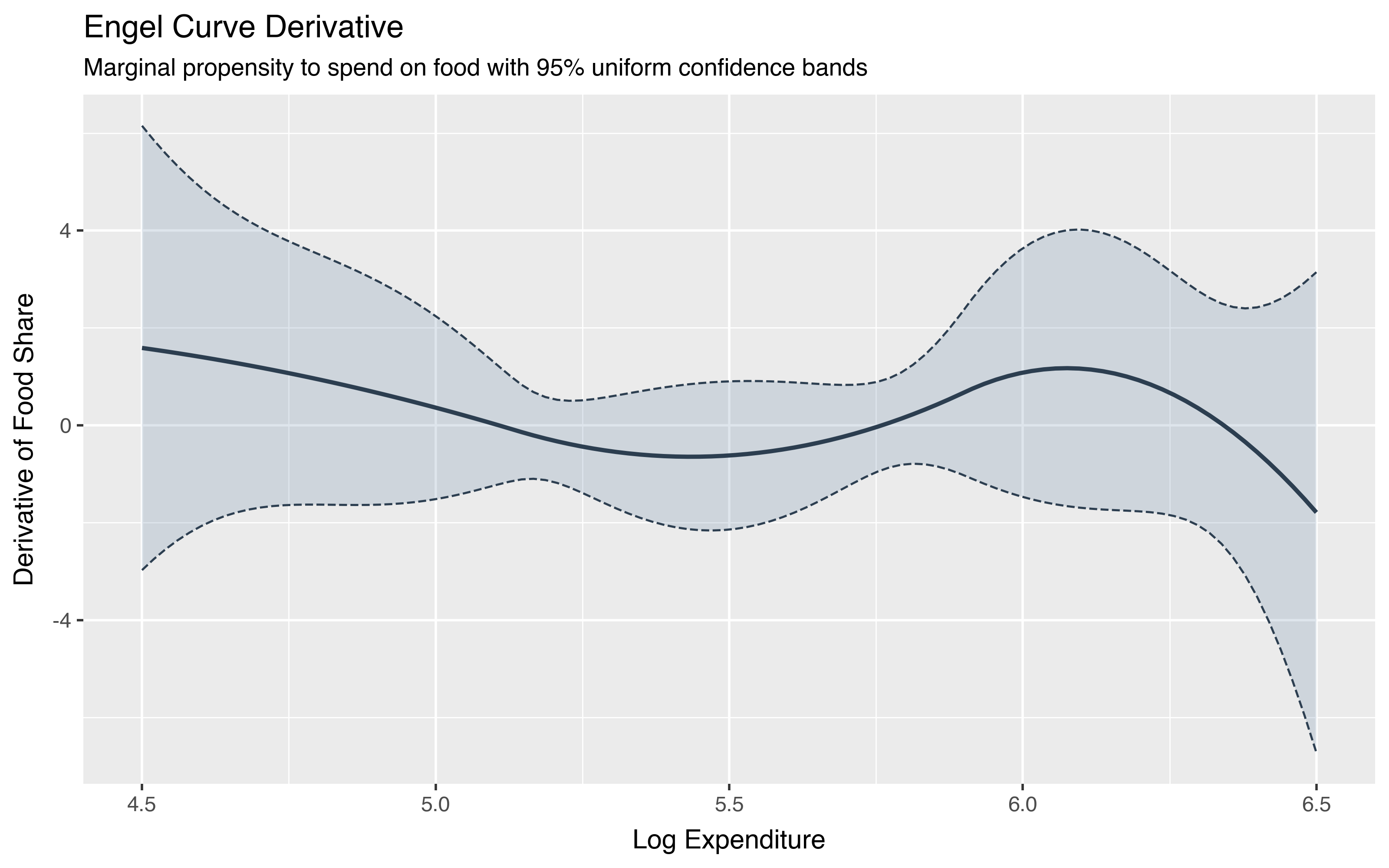
The derivative fluctuates around zero over the interior of the support. The
wider confidence bands for the derivative compared to the function estimate
reflect the additional uncertainty inherent in estimating slopes rather than
levels. To estimate higher-order derivatives or derivatives with respect to a
different variable in the multivariate case, use the deriv_order and
deriv_index parameters.
Simulation with a known function#
With real data we never know the true curve, so it is hard to tell how well the estimator is performing. Simulations let us check by generating data from a known function and seeing whether the estimate recovers it. Here we use a deliberately wiggly regression function \(h_0(x) = \sin(15\pi x)\cos(x)\) to stress-test the data-driven dimension selection.
rng = np.random.default_rng(42)
n = 10000
X = rng.uniform(0, 1, n)
U = rng.normal(0, 1, n)
Y = np.sin(15 * np.pi * X) * np.cos(X) + U

X_eval = np.linspace(X.min(), X.max(), 100).reshape(-1, 1)
h0_true = np.sin(15 * np.pi * X_eval.ravel()) * np.cos(X_eval.ravel())

result_sim = did.npiv(
    y=Y, x=X.reshape(-1, 1), w=X.reshape(-1, 1),
    x_eval=X_eval,
    biters=200, seed=42,
)
print(f"Selected segments: {result_sim.j_x_segments}")
Selected segments: 32
The data-driven procedure selects 32 segments to accommodate the rapid oscillations. We can overlay the estimate and the true function to see how well they match.
from plotnine import scale_color_manual, guides, guide_legend

func_df = pl.DataFrame({
    "x": np.tile(X_eval.ravel(), 2),
    "y": np.concatenate([result_sim.h, h0_true]),
    "Line": ["Estimate"] * 100 + ["True function"] * 100,
}).to_pandas()
band_df = pl.DataFrame({
    "x": X_eval.ravel(),
    "Lower": result_sim.h_lower,
    "Upper": result_sim.h_upper,
}).to_pandas()

p = (
    ggplot()
    + geom_ribbon(band_df, aes(x="x", ymin="Lower", ymax="Upper"), alpha=0.2, fill="#5b7ea4")
    + geom_line(band_df, aes(x="x", y="Upper"), linetype="dashed", color="#2c3e50", size=0.4)
    + geom_line(band_df, aes(x="x", y="Lower"), linetype="dashed", color="#2c3e50", size=0.4)
    + geom_line(func_df, aes(x="x", y="y", color="Line"), size=0.8)
    + scale_color_manual(values={"Estimate": "#2c3e50", "True function": "#c0392b"})
    + labs(
        x="X",
        y="h(X)",
        title="Estimated vs True Regression Function",
        subtitle="Data-driven NPIV with 95% uniform confidence bands (n = 10,000)",
    )
    + theme_gray()
    + theme(
        legend_position="bottom",
        plot_title=element_text(size=13, weight="bold"),
        plot_subtitle=element_text(size=10),
    )
    + guides(color=guide_legend(title=""))
)
p.save("plot_npiv_sim_function.png", dpi=200, width=8, height=5)
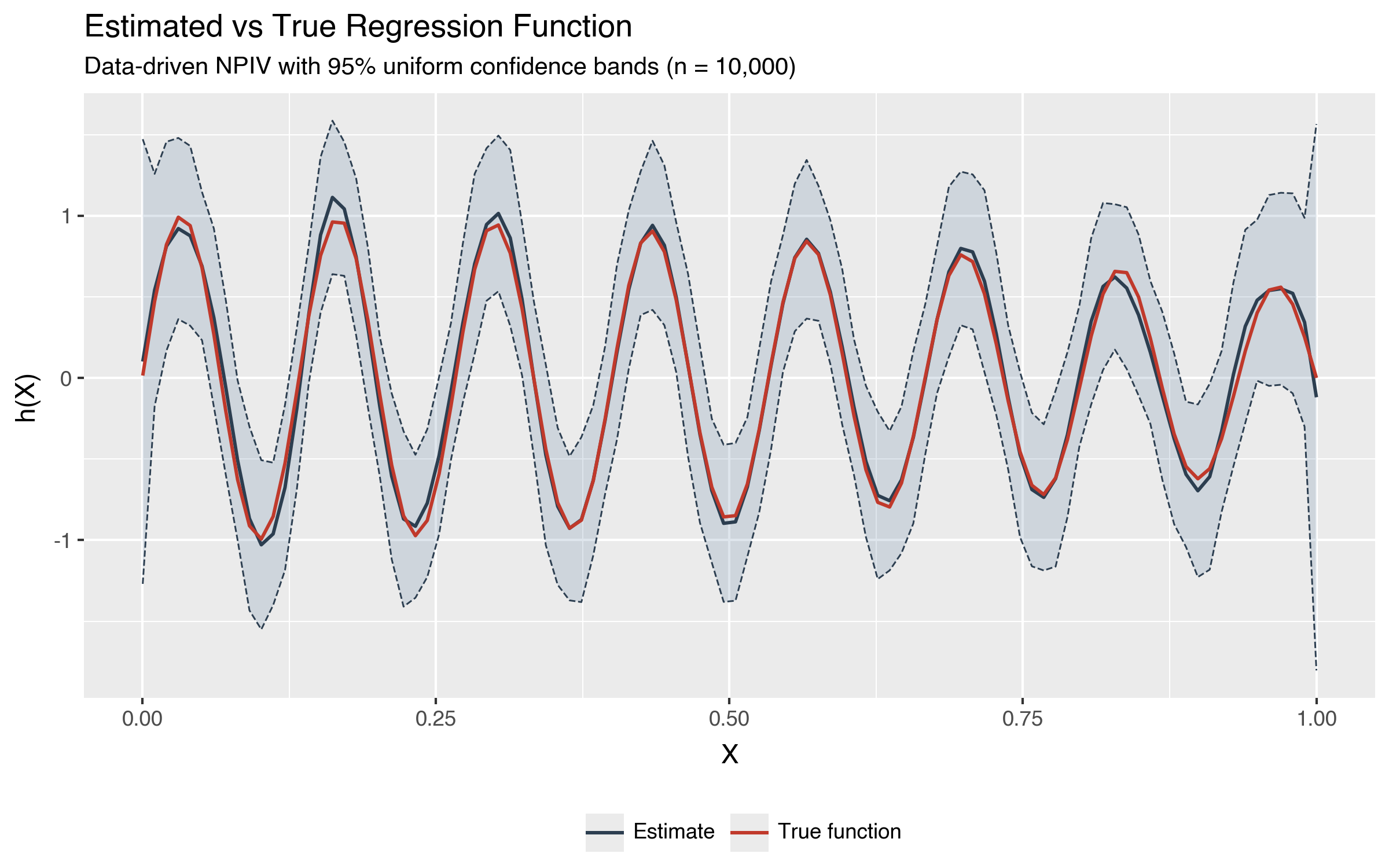
The estimate (dark line) tracks the true function (red line) closely, and the true function lies within the 95% uniform confidence bands everywhere. The data-driven procedure automatically chose enough basis functions to capture the rapid oscillations without over-fitting.
We can do the same comparison for the derivative \(h_0'(x) = 15\pi\cos(15\pi x)\cos(x) - \sin(x)\sin(15\pi x)\).
d0_true = (
    15 * np.pi * np.cos(15 * np.pi * X_eval.ravel()) * np.cos(X_eval.ravel())
    - np.sin(X_eval.ravel()) * np.sin(15 * np.pi * X_eval.ravel())
)

deriv_df = pl.DataFrame({
    "x": np.tile(X_eval.ravel(), 2),
    "y": np.concatenate([result_sim.deriv, d0_true]),
    "Line": ["Estimate"] * 100 + ["True derivative"] * 100,
}).to_pandas()
deriv_band_df = pl.DataFrame({
    "x": X_eval.ravel(),
    "Lower": result_sim.h_lower_deriv,
    "Upper": result_sim.h_upper_deriv,
}).to_pandas()

p = (
    ggplot()
    + geom_ribbon(deriv_band_df, aes(x="x", ymin="Lower", ymax="Upper"), alpha=0.2, fill="#5b7ea4")
    + geom_line(deriv_band_df, aes(x="x", y="Upper"), linetype="dashed", color="#2c3e50", size=0.4)
    + geom_line(deriv_band_df, aes(x="x", y="Lower"), linetype="dashed", color="#2c3e50", size=0.4)
    + geom_line(deriv_df, aes(x="x", y="y", color="Line"), size=0.8)
    + scale_color_manual(values={"Estimate": "#2c3e50", "True derivative": "#c0392b"})
    + labs(
        x="X",
        y="h'(X)",
        title="Estimated vs True Derivative",
        subtitle="Data-driven NPIV with 95% uniform confidence bands (n = 10,000)",
    )
    + theme_gray()
    + theme(
        legend_position="bottom",
        plot_title=element_text(size=13, weight="bold"),
        plot_subtitle=element_text(size=10),
    )
    + guides(color=guide_legend(title=""))
)
p.save("plot_npiv_sim_deriv.png", dpi=200, width=8, height=5)
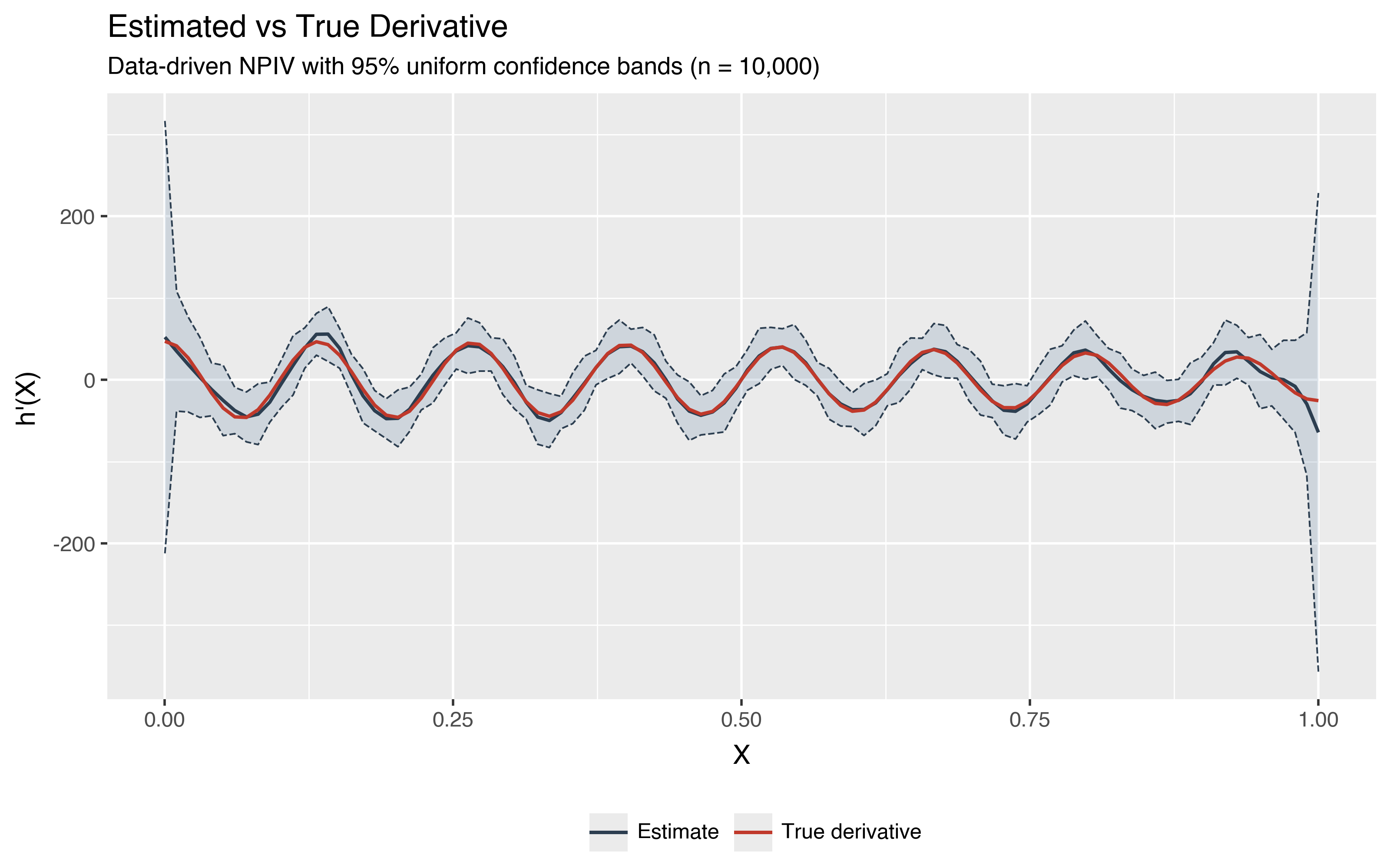
The derivative estimate recovers the oscillating pattern of the true derivative over the interior of the support. The confidence bands are wider than for the function estimate because derivatives amplify noise. Near the boundaries of the support the estimate deteriorates, which is typical for nonparametric methods with limited data at the edges.
Data-driven dimension selection#
Choosing the right number of B-spline segments involves a trade-off. Too few segments and the estimate is too rigid to capture the true shape. Too many and the estimate becomes noisy, especially with instrumental variables where the estimation problem is ill-posed.
When j_x_segments is omitted, npiv automatically
selects the sieve dimension using the Lepski method
(npiv_j). This data-driven
procedure adapts to the unknown smoothness of the structural function and the
strength of the instruments, achieving the minimax convergence rate without
requiring the researcher to tune any parameters.
result_dd = did.npiv(
    data=df,
    yname="food",
    xname="logexp",
    wname="logwages",
    biters=200,
    seed=42,
)
print(f"Selected segments: {result_dd.j_x_segments}")
print(f"Adaptive UCB critical value: {result_dd.cv:.3f}")
Selected segments: 1
Adaptive UCB critical value: 4.768
The adaptive critical value is larger than the fixed-dimension critical value
because it accounts for the additional uncertainty from dimension selection.
The resulting confidence bands are honest (guaranteed coverage over a class of
data-generating processes) and adaptive (contract at the minimax rate), making
them more efficient than the undersmoothing approach used with a fixed
j_x_segments.
Estimation without confidence bands#
When you only need point estimates and want to skip the bootstrap, set
ucb_h=False and ucb_deriv=False. This is substantially faster and
useful for exploratory analysis.
result_fast = did.npiv(
    data=df,
    yname="food",
    xname="logexp",
    wname="logwages",
    j_x_segments=5,
    ucb_h=False,
    ucb_deriv=False,
)
print(f"h_lower is {result_fast.h_lower}")
h_lower is None
This calls npiv_est internally, the core TSLS estimator
without bootstrap inference.
Using numpy arrays#
Instead of a DataFrame, you can also pass numpy arrays directly.
y = df["food"].to_numpy()
x = df["logexp"].to_numpy().reshape(-1, 1)
w = df["logwages"].to_numpy().reshape(-1, 1)

result_arr = did.npiv(y=y, x=x, w=w, j_x_segments=5, biters=200, seed=42)
The DataFrame and array interfaces produce identical results. The DataFrame interface additionally accepts any object implementing the Arrow PyCapsule Interface, including pandas, pyarrow Table, and cudf DataFrames.
Choosing the basis type#
For multivariate regressors, the basis parameter controls how marginal
B-spline bases are combined.
tensor constructs the full tensor product of univariate bases. This is the most flexible but the dimension grows exponentially with the number of regressors.
additive restricts the model to an additive structure \(h_0(x) = \sum_i h_i(x_i)\). The dimension grows linearly.
glp (generalized linear product) includes main effects and selected interactions, providing a middle ground.
With a single regressor, all three produce the same result. The distinction matters only for multivariate \(X\).
Knot placement#
The knots parameter controls whether B-spline knots are placed uniformly
across the support ("uniform", the default) or at empirical quantiles of
the data ("quantiles"). Quantile knots place more basis functions where
data is dense, which can improve estimates in those regions at the cost of
less resolution in sparse areas.