Continuous Difference-in-Differences#
Treatment intensity often varies continuously. A state might expand Medicaid to 138% of the federal poverty level while another expands to 200%. A job training program might provide 20 hours of instruction to some participants and 100 hours to others. Binary treatment comparisons throw away this rich variation in dosage.
The Callaway, Goodman-Bacon, and Sant’Anna (2024) estimator recovers dose-response functions showing how average treatment effects vary with treatment intensity. It handles both continuous doses and staggered adoption, allowing researchers to trace out the full relationship between treatment intensity and outcomes.
See also
Introduction to DiD for background on the parallel trends assumption and potential outcomes framework, and DiD with Continuous Treatments for the theoretical foundations behind this estimator.
Simulating data#
For this walkthrough, we use simulated panel data where treatment intensity varies continuously and adoption is staggered across time periods.
import moderndid as did

data = did.gen_cont_did_data(
    n=2000,
    num_time_periods=4,
    dose_linear_effect=0.5,
    dose_quadratic_effect=0.3,
    seed=1234,
)
print(data.head(10))
shape: (10, 5)
┌─────┬─────┬──────────┬─────────────┬──────────┐
│ id  ┆ G   ┆ D        ┆ time_period ┆ Y        │
│ --- ┆ --- ┆ ---      ┆ ---         ┆ ---      │
│ i64 ┆ i64 ┆ f64      ┆ i64         ┆ f64      │
╞═════╪═════╪══════════╪═════════════╪══════════╡
│ 1   ┆ 4   ┆ 0.780114 ┆ 1           ┆ 3.151232 │
│ 1   ┆ 4   ┆ 0.780114 ┆ 2           ┆ 5.835213 │
│ 1   ┆ 4   ┆ 0.780114 ┆ 3           ┆ 6.435796 │
│ 1   ┆ 4   ┆ 0.780114 ┆ 4           ┆ 8.272636 │
│ 2   ┆ 2   ┆ 0.734603 ┆ 1           ┆ 2.355389 │
│ 2   ┆ 2   ┆ 0.734603 ┆ 2           ┆ 5.59693  │
│ 2   ┆ 2   ┆ 0.734603 ┆ 3           ┆ 5.066891 │
│ 2   ┆ 2   ┆ 0.734603 ┆ 4           ┆ 6.797199 │
│ 3   ┆ 4   ┆ 0.40841  ┆ 1           ┆ 6.236491 │
│ 3   ┆ 4   ┆ 0.40841  ┆ 2           ┆ 5.606803 │
└─────┴─────┴──────────┴─────────────┴──────────┘
The data has 2,000 units observed across 4 time periods. Each unit has a
treatment dose D that is continuous and time-invariant. The timing group
G indicates when treatment begins, with 0 for never-treated units. In this
simulation, the true dose-response function has both linear (0.5) and quadratic
(0.3) components, so effects increase with dose at an accelerating rate.
Important data conventions for continuous treatments include setting the dose to its eventual value even in pre-treatment periods for treated units. This keeps the treatment definition consistent across time. Never-treated units should have dose values of zero in all periods.
Estimating dose-response functions#
With continuous treatments, we are interested in dose-response functions that
show how average treatment effects vary with treatment intensity. The
cont_did function estimates these using B-spline basis functions that
flexibly approximate the dose-response curve.
result = did.cont_did(
    data=data,
    yname="Y",
    tname="time_period",
    idname="id",
    dname="D",
    gname="G",
    target_parameter="level",
    aggregation="dose",
    degree=3,
    num_knots=1,
    biters=100,
    cband=True,
)
print(result)
==============================================================================
 Continuous Treatment Dose-Response Results
==============================================================================

 Overall ATT:

┌────────┬────────────┬────────────────────────┐
│    ATT │ Std. Error │ [95% Conf. Interval]   │
├────────┼────────────┼────────────────────────┤
│ 0.3824 │     0.0917 │ [  0.2026,   0.5621] * │
└────────┴────────────┴────────────────────────┘

 Overall ACRT:

┌────────┬────────────┬────────────────────────┐
│   ACRT │ Std. Error │ [95% Conf. Interval]   │
├────────┼────────────┼────────────────────────┤
│ 0.7019 │     0.0784 │ [  0.5483,   0.8555] * │
└────────┴────────────┴────────────────────────┘

------------------------------------------------------------------------------
 Signif. codes: '*' confidence band does not cover 0

------------------------------------------------------------------------------
 Data Info
------------------------------------------------------------------------------
 Control Group: Not Yet Treated
 Anticipation Periods: 0

------------------------------------------------------------------------------
 Estimation Details
------------------------------------------------------------------------------
 Estimation Method: Parametric (B-spline)
 Spline Degree: 3
 Number of Knots: 1

------------------------------------------------------------------------------
 Inference
------------------------------------------------------------------------------
 Significance level: 0.05
 Bootstrap standard errors
==============================================================================
 Reference: Callaway et al. (2024)
Two key quantities stand out here. The Overall ATT is the average treatment effect across all treated units, weighted by the distribution of doses in the population. The Overall ACRT (Average Causal Response on the Treated) measures the average marginal effect of increasing the dose, essentially the slope of the dose-response curve.
Since we set the true linear effect to 0.5 and the quadratic effect to 0.3, we expect positive values for both the ATT and ACRT. The estimates confirm this, showing significant positive effects.
The degree and num_knots parameters control the flexibility of the
B-spline approximation. Higher values allow more complex dose-response shapes
but increase variance. With degree=3 and num_knots=1, we use a cubic
spline with one interior knot.
Understanding ATT versus ACRT#
Which estimate you should target depends on your research question.
ATT(d) estimates the average effect of receiving dose \(d\) compared to no treatment.
Level of the dose-response curve at each point
For policy evaluation, tells you the expected benefit of a specific treatment intensity
Identified under standard parallel trends
Recovers \(ATT(d)\), a local effect for units who received dose \(d\)
ACRT(d) estimates the marginal effect of increasing the dose.
Derivative (slope) of the dose-response curve
For policy optimization, tells you whether increasing intensity yields additional benefits
Identified under strong parallel trends (typically stronger)
Recovers \(ATE(d)\) and \(ACRT(d)\) as population-level parameters
Both parameters come from the same underlying comparison, the change in outcomes for dose group \(d\) minus the change for untreated units. What differs is the causal interpretation. Under standard parallel trends, this comparison identifies \(ATT(d)\), a local effect specific to units who actually received dose \(d\). Under strong parallel trends, it also identifies \(ATE(d)\), the effect for the general population, and \(ACRT(d)\) gains a causal interpretation as the derivative of this curve.
When the dose-response is linear, ATT and ACRT have a simple relationship because the slope is constant. With our quadratic specification, the ACRT varies with dose, being larger at higher doses where the curve is steeper.
When can you trust each estimate?#
ATT and ACRT require different identifying assumptions, so which one you report depends on both your research question and what you are willing to assume.
ATT(d) and standard parallel trends
This is the same assumption as in binary DiD extended to the continuous case. We assume that untreated potential outcomes would have evolved similarly across dose groups. If you believe that absent treatment, high-dose and low-dose units would have followed parallel outcome paths, ATT(d) is identified. This is the right target when you want to know the effect of receiving dose d versus no treatment.
ACRT(d) and strong parallel trends
This is a typically stronger assumption than standard parallel trends (the two are technically non-nested, but in practice strong parallel trends is the more demanding condition). Standard parallel trends alone is not enough because comparing outcomes across dose groups mixes together the true causal response with a selection bias term. Even if untreated potential outcomes evolve identically, the observed outcome paths of different dose groups can diverge because units who chose different doses may experience different treatment effects from the same dose.
Strong parallel trends eliminates this selection bias by ruling out systematic treatment effect heterogeneity across dose groups.
When combined with standard parallel trends, it is equivalent to assuming \(ATT(d) = ATE(d)\) for all \(d\), meaning the effect of dose \(d\) on units who chose that dose equals its effect on the general population
This rules out selection on gains, where units that benefit more from treatment systematically choose higher doses
ACRT is the right target when you want the marginal benefit of increasing dose, but you should be explicit that this requires assuming away selection on gains
Consider whether units in your setting plausibly sort into doses based on expected benefits. When dose is assigned by policy rules or randomization rather than chosen by units, strong parallel trends is more defensible.
Important
Flat pre-treatment estimates are consistent with standard parallel trends, but they say nothing about whether strong parallel trends holds. Pre-treatment periods only involve untreated potential outcomes, while strong parallel trends restricts how treated potential outcomes vary across dose groups.
For the full theoretical treatment of these assumptions, see the Background on Continuous DiD.
Event study aggregation#
While dose aggregation reveals how effects vary with treatment intensity, you might also want to see how effects evolve over time. Event study aggregation averages across doses while preserving the temporal structure, making it useful for examining treatment dynamics.
event_study = did.cont_did(
    data=data,
    yname="Y",
    tname="time_period",
    idname="id",
    dname="D",
    gname="G",
    target_parameter="level",
    aggregation="eventstudy",
    degree=3,
    num_knots=1,
    biters=100,
    cband=True,
)
print(event_study)
==============================================================================
 Aggregate Treatment Effects (Event Study)
==============================================================================

 Overall summary of ATT's:

┌────────┬────────────┬────────────────────────┐
│    ATT │ Std. Error │ [95% Conf. Interval]   │
├────────┼────────────┼────────────────────────┤
│ 0.4382 │     0.0494 │ [  0.3413,   0.5350] * │
└────────┴────────────┴────────────────────────┘


 Event time Effects:

┌────────────┬──────────┬────────────┬──────────────────────────┐
│ Event time │ Estimate │ Std. Error │ [95% Simult. Conf. Band] │
├────────────┼──────────┼────────────┼──────────────────────────┤
│         -2 │   0.0764 │     0.0805 │ [-0.1358,  0.2886]       │
│         -1 │   0.0300 │     0.0631 │ [-0.1364,  0.1964]       │
│          0 │   0.4536 │     0.0394 │ [ 0.3496,  0.5576] *     │
│          1 │   0.4118 │     0.0591 │ [ 0.2559,  0.5676] *     │
│          2 │   0.4492 │     0.0811 │ [ 0.2353,  0.6630] *     │
└────────────┴──────────┴────────────┴──────────────────────────┘

------------------------------------------------------------------------------
 Signif. codes: '*' confidence band does not cover 0

------------------------------------------------------------------------------
 Data Info
------------------------------------------------------------------------------
 Control Group: Not Yet Treated
 Anticipation Periods: 0

------------------------------------------------------------------------------
 Estimation Details
------------------------------------------------------------------------------
 Estimation Method: att

------------------------------------------------------------------------------
 Inference
------------------------------------------------------------------------------
 Significance level: 0.05
 Bootstrap standard errors
==============================================================================
 Reference: Callaway et al. (2024)
We can see the pre-treatment and post-treatment dynamics here. Event times -2 and -1 are pre-treatment periods that serve as placebo tests for parallel trends. Both estimates are close to zero and statistically insignificant, which is reassuring for the identifying assumption.
At event time 0 (the year of treatment adoption), effects appear immediately and remain stable in subsequent periods. This instantaneous and persistent effect pattern is consistent with our simulation design where the dose-response relationship is constant over time.
To examine how the marginal effect (ACRT) evolves over time instead of the
level effect (ATT), set target_parameter="slope".
event_study_slope = did.cont_did(
    data=data,
    yname="Y",
    tname="time_period",
    idname="id",
    dname="D",
    gname="G",
    target_parameter="slope",
    aggregation="eventstudy",
    degree=3,
    num_knots=1,
    biters=100,
    cband=True,
)
print(event_study_slope)
==============================================================================
 Aggregate Treatment Effects (Event Study)
==============================================================================

 Overall summary of ACRT's:

┌────────┬────────────┬────────────────────────┐
│   ACRT │ Std. Error │ [95% Conf. Interval]   │
├────────┼────────────┼────────────────────────┤
│ 0.5602 │     0.0944 │ [  0.3752,   0.7452] * │
└────────┴────────────┴────────────────────────┘


 Event time Effects:

┌────────────┬──────────┬────────────┬──────────────────────────┐
│ Event time │ Estimate │ Std. Error │ [95% Simult. Conf. Band] │
├────────────┼──────────┼────────────┼──────────────────────────┤
│         -2 │  -0.0097 │     0.0886 │ [-0.2006,  0.1812]       │
│         -1 │   0.3052 │     0.1341 │ [ 0.0165,  0.5938] *     │
│          0 │   0.7632 │     0.0976 │ [ 0.5530,  0.9735] *     │
│          1 │   0.2119 │     0.0993 │ [-0.0020,  0.4258]       │
│          2 │   0.7054 │     0.1757 │ [ 0.3271,  1.0837] *     │
└────────────┴──────────┴────────────┴──────────────────────────┘

------------------------------------------------------------------------------
 Signif. codes: '*' confidence band does not cover 0

------------------------------------------------------------------------------
 Data Info
------------------------------------------------------------------------------
 Control Group: Not Yet Treated
 Anticipation Periods: 0

------------------------------------------------------------------------------
 Estimation Details
------------------------------------------------------------------------------
 Estimation Method: dose

------------------------------------------------------------------------------
 Inference
------------------------------------------------------------------------------
 Significance level: 0.05
 Bootstrap standard errors
==============================================================================
 Reference: Callaway et al. (2024)
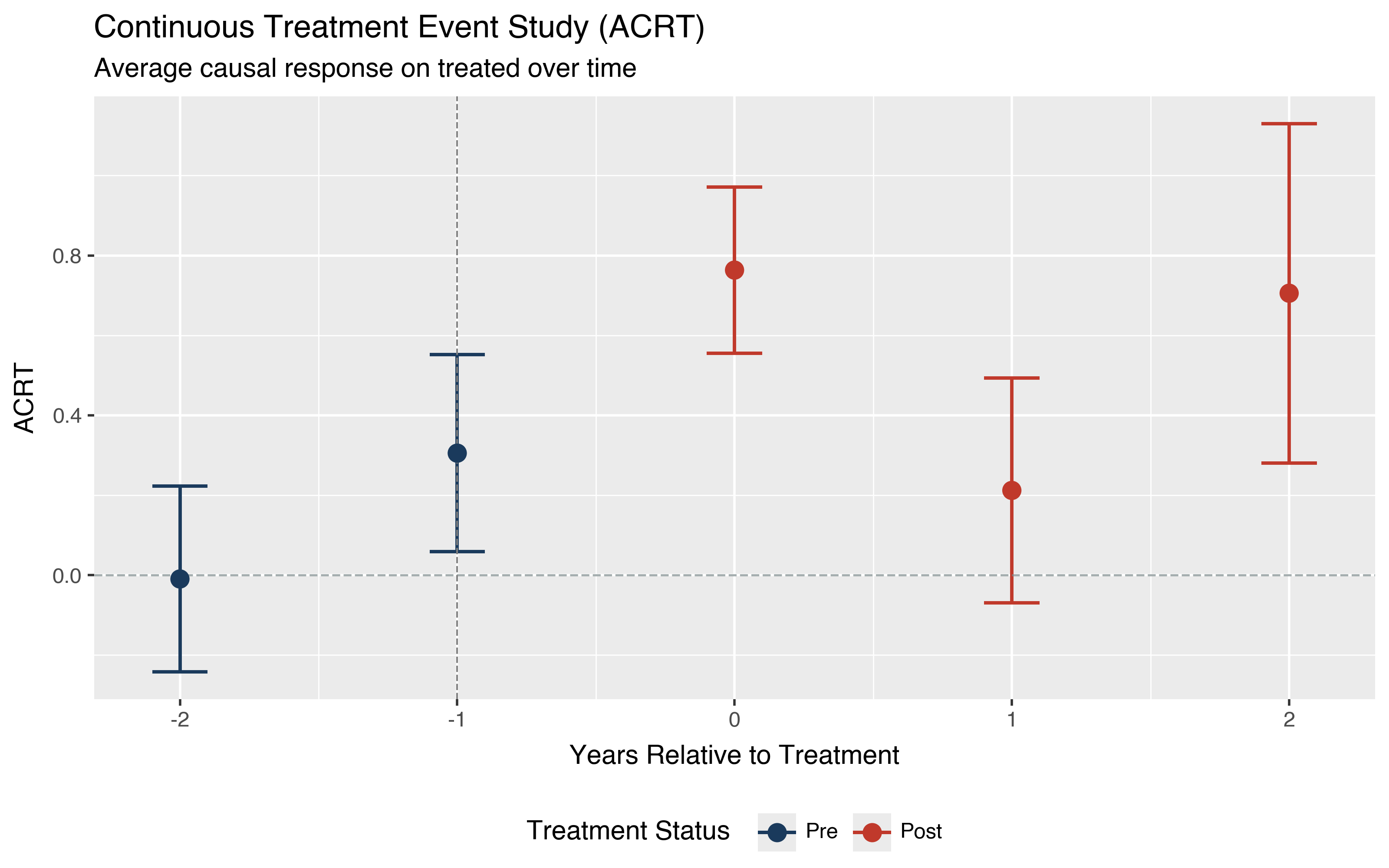
The ACRT event study shows how the marginal effect of increasing dose evolves
over time. The target_parameter setting only affects event study aggregation.
For dose aggregation, both the \(ATT(d)\) and \(ACRT(d)\) estimates are always computed and reported
regardless of this setting.
from plotnine import labs, theme, theme_gray

p = did.plot_event_study(event_study_slope, ref_period=-1)
p = (p
    + labs(
        x="Years Relative to Treatment",
        y="ACRT",
        title="Continuous Treatment Event Study (ACRT)",
        subtitle="Average causal response on treated over time",
    )
    + theme_gray()
    + theme(legend_position="bottom")
)
p.save("plot_cont_event_study_slope.png", dpi=200, width=8, height=5)
Plotting results#
Now we can visualize the dose-response curves to better understand the shape of the treatment effect function.
p = did.plot_dose_response(result, effect_type="att")
p = (p
    + labs(
        x="Treatment Dose",
        y="ATT(d)",
        title="Dose-Response Function",
        subtitle="Average treatment effect on treated by dose level",
    )
    + theme_gray()
    + theme(legend_position="bottom")
)
p.save("plot_cont_dose_att.png", dpi=200, width=8, height=5)
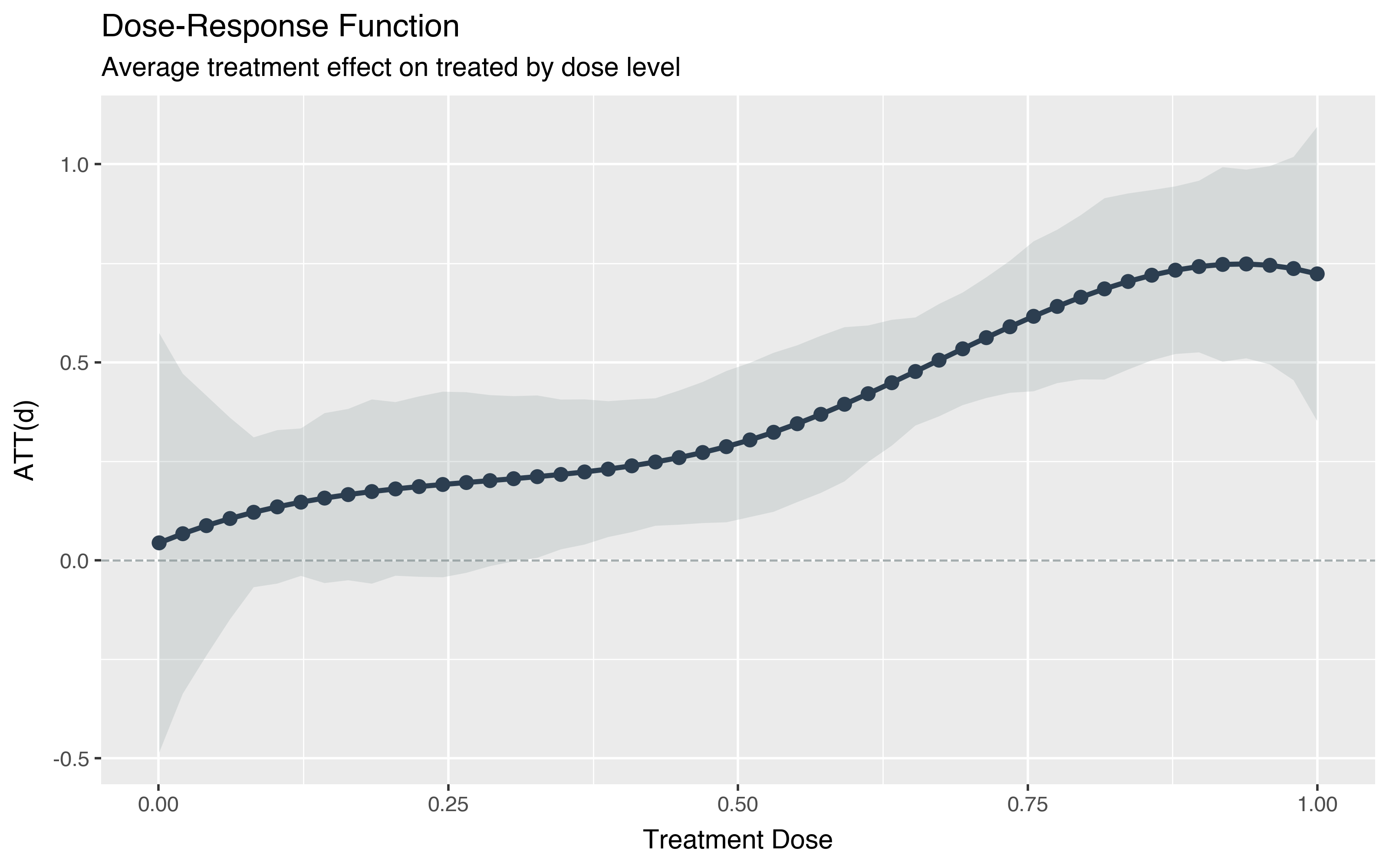
The dose-response plot shows the \(ATT(d)\) estimate as a function of dose, with pointwise confidence bands. Each point on this curve is identified under standard parallel trends, but interpreting the shape of the curve (comparing effects across different doses) requires the stronger parallel trends assumption discussed above. The widening bands at higher doses reflect increased uncertainty where fewer observations are available.
p = did.plot_dose_response(result, effect_type="acrt")
p = (p
    + labs(
        x="Treatment Dose",
        y="ACRT(d)",
        title="Marginal Dose-Response Function",
        subtitle="Average causal response on treated by dose level",
    )
    + theme_gray()
    + theme(legend_position="bottom")
)
p.save("plot_cont_dose_acrt.png", dpi=200, width=8, height=5)
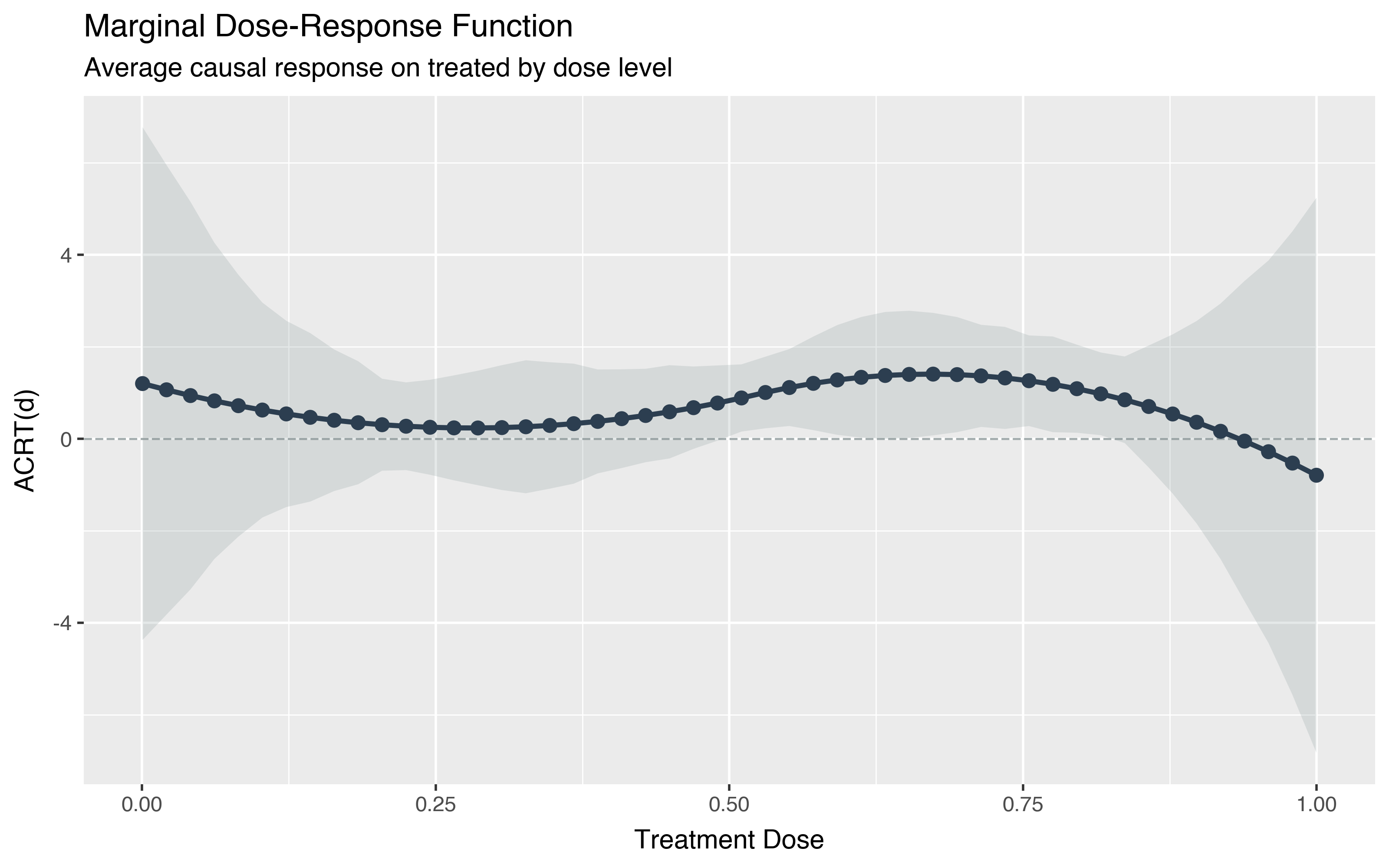
The \(ACRT(d)\) plot shows how the marginal effect varies with dose. The positive and increasing pattern indicates that higher doses yield not just larger effects but also larger marginal effects, consistent with our quadratic specification.
For the event study aggregation, use the standard event study plot.
p = did.plot_event_study(event_study, ref_period=-1)
p = (p
    + labs(
        x="Years Relative to Treatment",
        y="ATT",
        title="Continuous Treatment Event Study (ATT)",
        subtitle="Average treatment effect on treated over time",
    )
    + theme_gray()
    + theme(legend_position="bottom")
)
p.save("plot_cont_event_study.png", dpi=200, width=8, height=5)
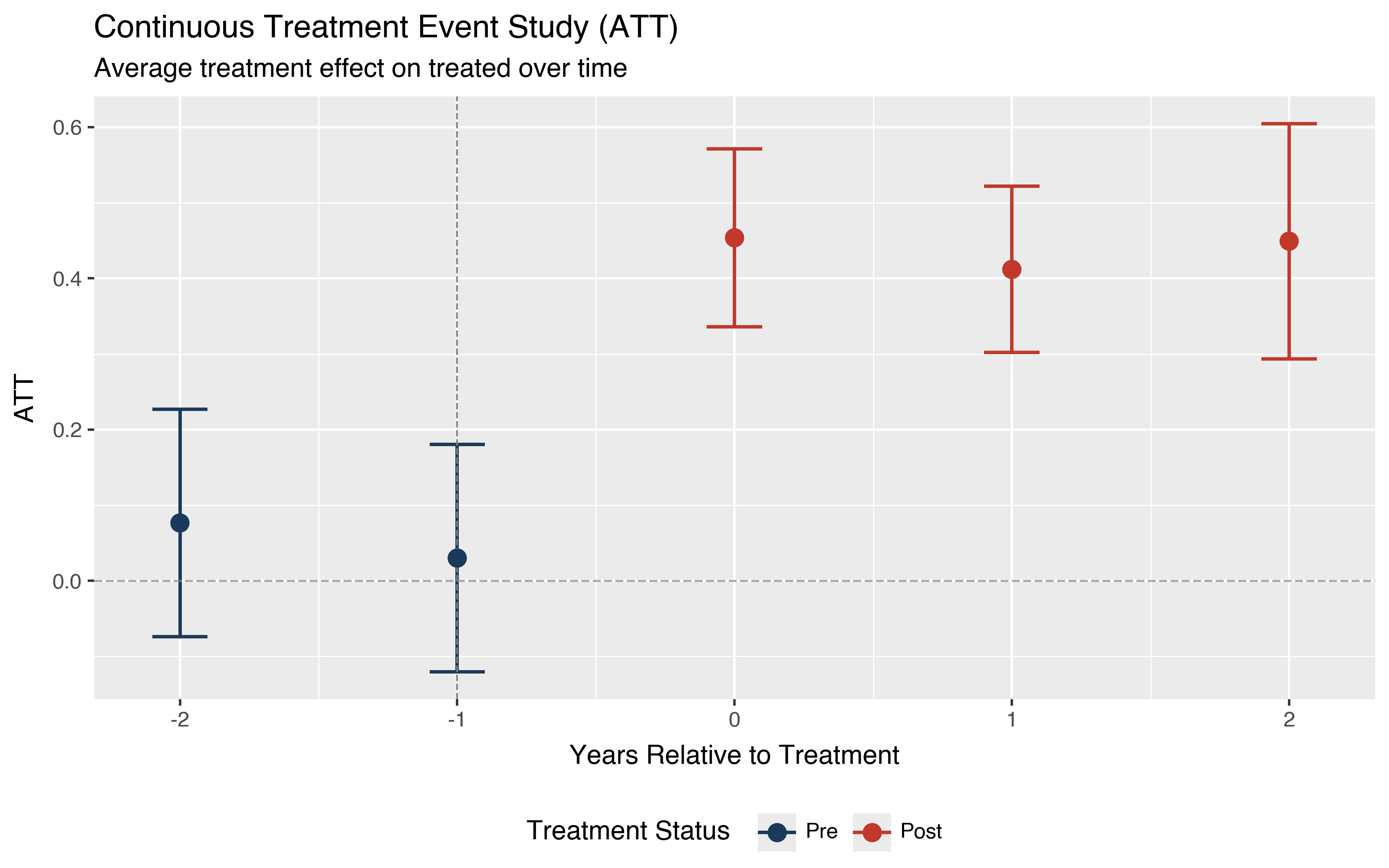
The event study visualization clearly shows the flat pre-treatment estimates and the immediate jump at event time 0. The flat pre-trends are consistent with the parallel trends assumption, and the sharp jump confirms a treatment effect.
Nonparametric estimation with CCK#
If you are unsure about the functional form of the dose-response, the
parametric B-spline specification may be too restrictive. The
dose_est_method="cck" option activates a nonparametric estimator based on
Chen, Christensen, and Kankanala (2024).
This approach makes minimal assumptions about the dose-response shape.
The CCK estimator is currently implemented for two-period settings without staggered adoption. For longer panels, you can collapse to two periods by averaging pre-treatment and post-treatment outcomes.
# Simulate two-period data for CCK
data_cck = did.gen_cont_did_data(
    n=2000,
    num_time_periods=2,
    dose_linear_effect=0,
    dose_quadratic_effect=1.0,
    seed=1234,
)

result_cck = did.cont_did(
    data=data_cck,
    yname="Y",
    tname="time_period",
    idname="id",
    dname="D",
    gname="G",
    target_parameter="level",
    aggregation="dose",
    dose_est_method="cck",
    biters=100,
    cband=True,
)
print(result_cck)
==============================================================================
 Continuous Treatment Dose-Response Results
==============================================================================

 Overall ATT:

┌────────┬────────────┬────────────────────────┐
│    ATT │ Std. Error │ [95% Conf. Interval]   │
├────────┼────────────┼────────────────────────┤
│ 0.3403 │     0.0677 │ [  0.2076,   0.4730] * │
└────────┴────────────┴────────────────────────┘

 Overall ACRT:

┌────────┬────────────┬────────────────────────┐
│   ACRT │ Std. Error │ [95% Conf. Interval]   │
├────────┼────────────┼────────────────────────┤
│ 0.7436 │     0.2919 │ [  0.1714,   1.3157] * │
└────────┴────────────┴────────────────────────┘

------------------------------------------------------------------------------
 Signif. codes: '*' confidence band does not cover 0

------------------------------------------------------------------------------
 Data Info
------------------------------------------------------------------------------
 Control Group: Not Yet Treated
 Anticipation Periods: 0

------------------------------------------------------------------------------
 Estimation Details
------------------------------------------------------------------------------
 Estimation Method: Non-parametric (CCK)

------------------------------------------------------------------------------
 Inference
------------------------------------------------------------------------------
 Significance level: 0.05
 Bootstrap standard errors
==============================================================================
 Reference: Callaway et al. (2024)
With a purely quadratic true effect (dose_quadratic_effect=1.0 and no linear term), the CCK estimator correctly identifies a significant positive ATT. The nonparametric approach allows the data to determine the dose-response shape rather than imposing a parametric form.
p = did.plot_dose_response(result_cck, effect_type="att")
p = (p
    + labs(
        x="Treatment Dose",
        y="ATT(d)",
        title="Nonparametric Dose-Response Function",
        subtitle="CCK estimator with purely quadratic treatment effect",
    )
    + theme_gray()
    + theme(legend_position="bottom")
)
p.save("plot_cont_cck.png", dpi=200, width=8, height=5)
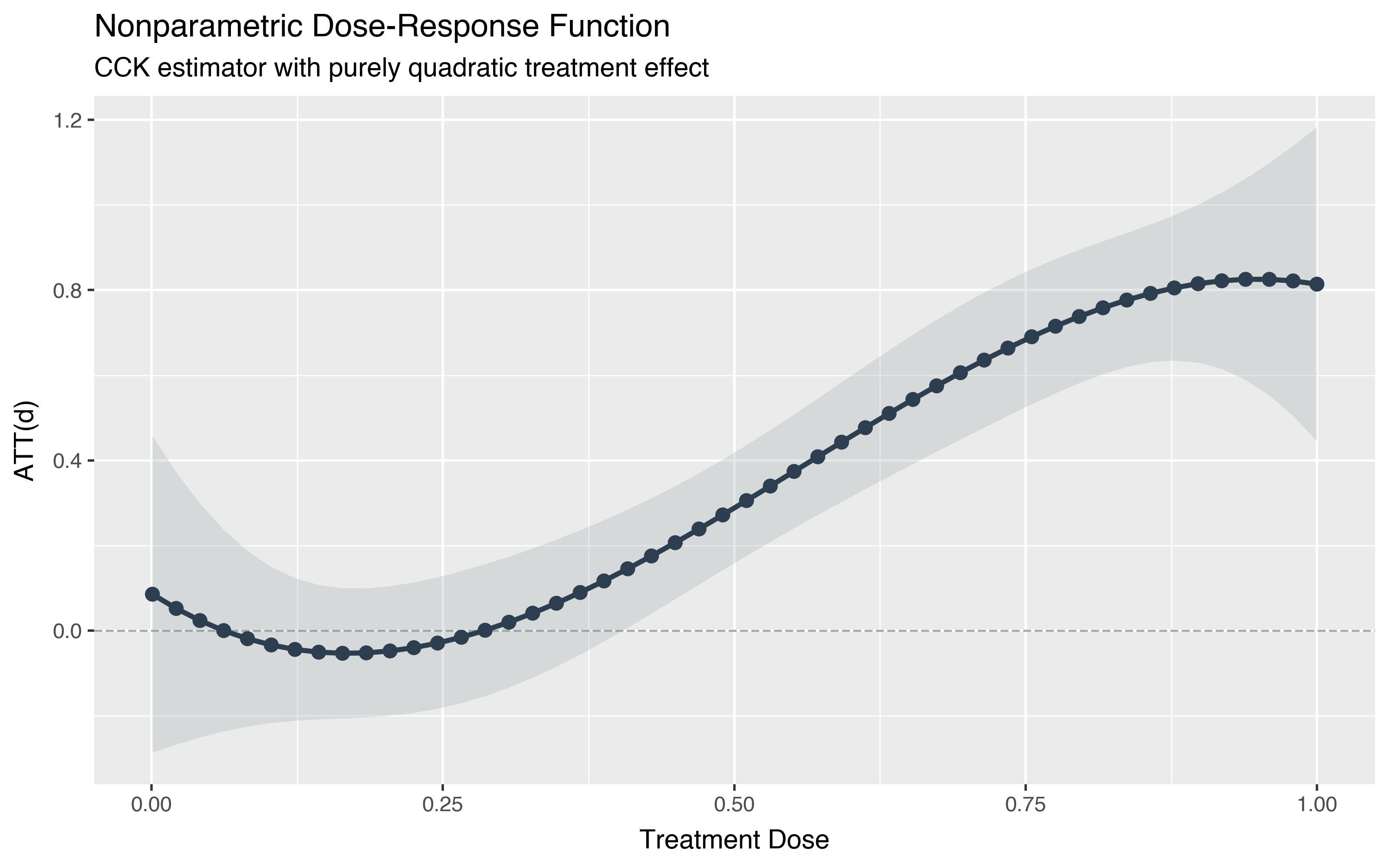
The nonparametric dose-response curve shows the characteristic quadratic shape, with effects accelerating as dose increases. The confidence bands are wider than the parametric version, reflecting the additional uncertainty from not assuming a functional form.
Control group options#
Like the standard staggered DiD estimator, the continuous treatment version supports different control group definitions.
Not Yet Treated (default) uses units that will eventually be treated but have not yet received treatment as controls. This maximizes the control pool but requires assuming that future treatment timing is unrelated to current potential outcomes.
Never Treated uses only units that never receive treatment during the sample period. This is more conservative and may be preferred when future treatment timing could be endogenous.
result_never = did.cont_did(
    data=data,
    yname="Y",
    tname="time_period",
    idname="id",
    dname="D",
    gname="G",
    target_parameter="level",
    aggregation="dose",
    control_group="nevertreated",
    degree=3,
    num_knots=1,
    biters=100,
    cband=True,
)
print(result_never)
==============================================================================
 Continuous Treatment Dose-Response Results
==============================================================================

 Overall ATT:

┌────────┬────────────┬────────────────────────┐
│    ATT │ Std. Error │ [95% Conf. Interval]   │
├────────┼────────────┼────────────────────────┤
│ 0.3871 │     0.0998 │ [  0.1916,   0.5827] * │
└────────┴────────────┴────────────────────────┘

 Overall ACRT:

┌────────┬────────────┬────────────────────────┐
│   ACRT │ Std. Error │ [95% Conf. Interval]   │
├────────┼────────────┼────────────────────────┤
│ 0.7019 │     0.0863 │ [  0.5327,   0.8711] * │
└────────┴────────────┴────────────────────────┘

------------------------------------------------------------------------------
 Signif. codes: '*' confidence band does not cover 0

------------------------------------------------------------------------------
 Data Info
------------------------------------------------------------------------------
 Control Group: Never Treated
 Anticipation Periods: 0

------------------------------------------------------------------------------
 Estimation Details
------------------------------------------------------------------------------
 Estimation Method: Parametric (B-spline)
 Spline Degree: 3
 Number of Knots: 1

------------------------------------------------------------------------------
 Inference
------------------------------------------------------------------------------
 Significance level: 0.05
 Bootstrap standard errors
==============================================================================
 Reference: Callaway et al. (2024)
With the never-treated control group, the point estimates are similar but standard errors are somewhat larger due to the smaller control pool. Which control group you choose depends on the empirical context and what assumptions you are most comfortable defending.
Next steps#
For details on additional estimation options including anticipation periods, base period selection, and bootstrap inference, see the Continuous DiD API reference.
For theoretical background on continuous treatment difference-in-differences, see the Background section.
For the binary-treatment version that this estimator generalizes, see the Staggered DiD walkthrough.