DiD with Intertemporal Treatment Effects#
Many treatments in applied work are neither binary nor permanent. A state might gradually phase in banking deregulation. A firm might adjust its training intensity over time. A country might strengthen or relax environmental regulations in response to political changes.
Standard difference-in-differences methods were not designed for these settings because they assume treatment is either on or off and stays on forever. Two-way fixed effects and local projection regressions can produce misleading results with time-varying treatments. Their coefficients are weighted sums of many different treatment effects, and the weights can be negative or can sum to less than one. At longer horizons the weights can even sum to a negative number, making effects appear to fade or reverse sign when the true effects are actually persistent.
The de Chaisemartin and D’Haultfoeuille (2024) estimator avoids these problems by comparing units whose treatment changed to those with the same baseline treatment that have not yet changed. This allows for valid causal inference even when treatment intensity varies and past treatments affect current outcomes.
See also
Introduction to DiD for background on the parallel trends assumption and potential outcomes framework, and DiD with Intertemporal Treatment Effects for the theoretical foundations behind this estimator.
Empirical application#
This example replicates the empirical analysis from de Chaisemartin and D’Haultfoeuille (2024), which revisits Favara and Imbs (2015).
In 1994, the Interstate Banking and Branching Efficiency Act (IBBEA) allowed US banks to operate across state borders without formal authorization from state authorities. However, states could still impose up to four restrictions on interstate branching. These included requiring explicit state approval for de novo branching, setting minimum age requirements for merger targets, prohibiting the acquisition of individual branches, and capping the statewide deposits controlled by a single bank. States lifted these restrictions at different times and in different combinations between 1994 and 2005, creating a non-binary, time-varying treatment.
The outcome of interest is the change in log volume of bank loans
(Dl_vloans_b), measuring the growth rate of mortgage lending at the
county level. The dataset contains 1,045 counties observed annually from
1994 to 2005, nested within states (state_n). The treatment
inter_bra indicates whether interstate branching was permitted. Of
the 1,045 counties, 916 eventually experience a change in deregulation
status and 129 never switch. Most states that deregulate do so for the
first time between 1995 and 1998.
Favara and Imbs (2015) originally concluded that deregulation had only short-lived effects on credit supply, based on local-projection coefficients that became small and insignificant at longer horizons. However, de Chaisemartin and D’Haultfoeuille (2024) show that this apparent fading was an artifact of the local-projection weights turning negative at longer horizons. Their estimator avoids these weighting problems and finds persistent effects of deregulation on lending.
Loading the data#
import moderndid as md

df = md.load_favara_imbs()
print(df.head(10))
shape: (10, 7)
┌──────┬────────┬─────────┬─────────────┬───────────┬──────────┬──────────┐
│ year ┆ county ┆ state_n ┆ Dl_vloans_b ┆ inter_bra ┆ w1       ┆ Dl_hpi   │
│ ---  ┆ ---    ┆ ---     ┆ ---         ┆ ---       ┆ ---      ┆ ---      │
│ i64  ┆ i64    ┆ i64     ┆ f64         ┆ i64       ┆ f64      ┆ f64      │
╞══════╪════════╪═════════╪═════════════╪═══════════╪══════════╪══════════╡
│ 1994 ┆ 1001   ┆ 1       ┆ 0.270248    ┆ 0         ┆ 0.975312 ┆ 0.003176 │
│ 1995 ┆ 1001   ┆ 1       ┆ -0.038427   ┆ 0         ┆ 0.975312 ┆ 0.048912 │
│ 1996 ┆ 1001   ┆ 1       ┆ 0.161633    ┆ 0         ┆ 0.975312 ┆ 0.058203 │
│ 1997 ┆ 1001   ┆ 1       ┆ 0.056523    ┆ 0         ┆ 0.975312 ┆ 0.044366 │
│ 1998 ┆ 1001   ┆ 1       ┆ 0.034236    ┆ 1         ┆ 0.975312 ┆ 0.047092 │
│ 1999 ┆ 1001   ┆ 1       ┆ 0.048719    ┆ 1         ┆ 0.975312 ┆ 0.00628  │
│ 2000 ┆ 1001   ┆ 1       ┆ -0.034618   ┆ 1         ┆ 0.975312 ┆ 0.018803 │
│ 2001 ┆ 1001   ┆ 1       ┆ -0.010966   ┆ 1         ┆ 0.975312 ┆ 0.068863 │
│ 2002 ┆ 1001   ┆ 1       ┆ 0.121278    ┆ 1         ┆ 0.975312 ┆ 0.060576 │
│ 2003 ┆ 1001   ┆ 1       ┆ 0.202691    ┆ 1         ┆ 0.975312 ┆ 0.024043 │
└──────┴────────┴─────────┴─────────────┴───────────┴──────────┴──────────┘
The first county in the output switched from no interstate branching
(inter_bra = 0) to permitted (inter_bra = 1) in 1998. In this
dataset, deregulation is one-directional since states lifted restrictions
but did not reimpose them. The estimator can also handle non-absorbing
treatments where reversals occur.
Estimation#
The estimator compares the outcome evolution of “switchers” (counties whose
treatment changes) to “non-switchers” with the same baseline treatment. The
effects parameter specifies how many post-treatment horizons to estimate.
result = md.did_multiplegt(
    data=df,
    yname="Dl_vloans_b",
    idname="county",
    tname="year",
    dname="inter_bra",
    effects=5,
    cluster="state_n",
)
print(result)
===============================================================================
 Intertemporal Treatment Effects
===============================================================================

 Average Total Effect:

┌────────┬────────────┬────────────────────────┬───────┬───────────┐
│    ATE │ Std. Error │ [95% Conf. Interval]   │     N │ Switchers │
├────────┼────────────┼────────────────────────┼───────┼───────────┤
│ 0.0346 │     0.0131 │ [  0.0090,   0.0602] * │ 12947 │      4525 │
└────────┴────────────┴────────────────────────┴───────┴───────────┘


 Treatment Effects by Horizon:

┌─────────┬──────────┬────────────┬────────────────────────┬──────┬───────────┐
│ Horizon │ Estimate │ Std. Error │ [95% Conf. Interval]   │    N │ Switchers │
├─────────┼──────────┼────────────┼────────────────────────┼──────┼───────────┤
│       1 │   0.0435 │     0.0353 │ [ -0.0257,   0.1127]   │ 3810 │       905 │
│       2 │   0.0387 │     0.0452 │ [ -0.0498,   0.1273]   │ 2990 │       905 │
│       3 │   0.0813 │     0.0494 │ [ -0.0155,   0.1781]   │ 2418 │       905 │
│       4 │   0.0706 │     0.0654 │ [ -0.0575,   0.1987]   │ 1929 │       905 │
│       5 │   0.1476 │     0.0657 │ [  0.0189,   0.2763] * │ 1800 │       905 │
└─────────┴──────────┴────────────┴────────────────────────┴──────┴───────────┘

-------------------------------------------------------------------------------
 Signif. codes: '*' confidence interval does not cover 0

-------------------------------------------------------------------------------
 Data Info
-------------------------------------------------------------------------------
 Number of units: 1045
 Switchers: 916
 Never-switchers: 129

-------------------------------------------------------------------------------
 Estimation Details
-------------------------------------------------------------------------------
 Effects estimated: 5
 Placebos estimated: 0

-------------------------------------------------------------------------------
 Inference
-------------------------------------------------------------------------------
 Confidence level: 95%
 Clustered standard errors: state_n
===============================================================================
 See de Chaisemartin and D'Haultfoeuille (2024) for details.
We can see treatment effects at each horizon (periods since the first treatment change). Effects are positive across all horizons and grow over time, reaching 0.15 at horizon 5. This growth pattern is consistent with deregulation having cumulative effects as banks gradually expand interstate operations and increase competitive lending. Individual horizon effects are imprecise (only horizon 5 is individually significant), but the statistically significant Average Total Effect of 0.035 indicates a meaningful overall impact of deregulation on lending.
The 905 switchers at each horizon represents the subset used for that specific comparison. The declining sample sizes at longer horizons (from 3,810 at horizon 1 to 1,800 at horizon 5) reflect the panel structure, since fewer switchers have enough post-treatment periods to contribute to later horizons. As a practical rule, you should only report effects at horizons where a substantial share of switchers contribute. If a horizon applies to only a small, unrepresentative subset of units, the estimate may not generalize. The same logic applies to placebos.
Adding placebo tests#
It is always good practice to check whether switchers and non-switchers had similar outcome trends before the treatment change. Significant pre-treatment effects would suggest a violation of parallel trends.
result = md.did_multiplegt(
    data=df,
    yname="Dl_vloans_b",
    idname="county",
    tname="year",
    dname="inter_bra",
    effects=5,
    placebo=3,
    cluster="state_n",
)
print(result)
===============================================================================
 Intertemporal Treatment Effects
===============================================================================

 Average Total Effect:

┌────────┬────────────┬────────────────────────┬───────┬───────────┐
│    ATE │ Std. Error │ [95% Conf. Interval]   │     N │ Switchers │
├────────┼────────────┼────────────────────────┼───────┼───────────┤
│ 0.0346 │     0.0131 │ [  0.0090,   0.0602] * │ 12947 │      4525 │
└────────┴────────────┴────────────────────────┴───────┴───────────┘


 Treatment Effects by Horizon:

┌─────────┬──────────┬────────────┬────────────────────────┬──────┬───────────┐
│ Horizon │ Estimate │ Std. Error │ [95% Conf. Interval]   │    N │ Switchers │
├─────────┼──────────┼────────────┼────────────────────────┼──────┼───────────┤
│       1 │   0.0435 │     0.0353 │ [ -0.0257,   0.1127]   │ 3810 │       905 │
│       2 │   0.0387 │     0.0452 │ [ -0.0498,   0.1273]   │ 2990 │       905 │
│       3 │   0.0813 │     0.0494 │ [ -0.0155,   0.1781]   │ 2418 │       905 │
│       4 │   0.0706 │     0.0654 │ [ -0.0575,   0.1987]   │ 1929 │       905 │
│       5 │   0.1476 │     0.0657 │ [  0.0189,   0.2763] * │ 1800 │       905 │
└─────────┴──────────┴────────────┴────────────────────────┴──────┴───────────┘


 Placebo Effects (Pre-treatment):

┌─────────┬──────────┬────────────┬────────────────────────┬──────┬───────────┐
│ Horizon │ Estimate │ Std. Error │ [95% Conf. Interval]   │    N │ Switchers │
├─────────┼──────────┼────────────┼────────────────────────┼──────┼───────────┤
│      -1 │   0.0548 │     0.0489 │ [ -0.0410,   0.1506]   │ 2777 │       896 │
│      -2 │  -0.0718 │     0.0654 │ [ -0.2001,   0.0564]   │ 1343 │       629 │
│      -3 │  -0.1095 │     0.0953 │ [ -0.2962,   0.0773]   │  895 │       489 │
└─────────┴──────────┴────────────┴────────────────────────┴──────┴───────────┘

 Joint test (placebos = 0): p-value = 0.1699

-------------------------------------------------------------------------------
 Signif. codes: '*' confidence interval does not cover 0

-------------------------------------------------------------------------------
 Data Info
-------------------------------------------------------------------------------
 Number of units: 1045
 Switchers: 916
 Never-switchers: 129

-------------------------------------------------------------------------------
 Estimation Details
-------------------------------------------------------------------------------
 Effects estimated: 5
 Placebos estimated: 3

-------------------------------------------------------------------------------
 Inference
-------------------------------------------------------------------------------
 Confidence level: 95%
 Clustered standard errors: state_n
===============================================================================
 See de Chaisemartin and D'Haultfoeuille (2024) for details.
The placebo effects at horizons -1, -2, and -3 are all statistically insignificant, with confidence intervals that include zero. The joint test p-value of 0.17 indicates we cannot reject the null that all pre-treatment effects are jointly zero at conventional levels. This is consistent with the parallel trends assumption, suggesting that counties that eventually deregulated were evolving similarly to those that had not yet deregulated (or never did), in the periods before deregulation occurred. The point estimates at placebos -2 and -3 are negative and somewhat large in absolute value, though imprecise. With more data, it would be worth investigating whether this reflects noise or a pre-existing divergence.
Normalized effects#
When treatment intensity varies across units, raw effects can be hard to interpret on their own. Normalized effects divide by the cumulative treatment change, giving you a per-unit-of-treatment interpretation.
result = md.did_multiplegt(
    data=df,
    yname="Dl_vloans_b",
    idname="county",
    tname="year",
    dname="inter_bra",
    effects=5,
    placebo=3,
    cluster="state_n",
    normalized=True,
    same_switchers=True,
    effects_equal=True,
)
print(result)
===============================================================================
 Intertemporal Treatment Effects
===============================================================================

 Average Total Effect:

┌────────┬────────────┬────────────────────────┬───────┬───────────┐
│    ATE │ Std. Error │ [95% Conf. Interval]   │     N │ Switchers │
├────────┼────────────┼────────────────────────┼───────┼───────────┤
│ 0.0346 │     0.0131 │ [  0.0090,   0.0602] * │ 12947 │      4525 │
└────────┴────────────┴────────────────────────┴───────┴───────────┘


 Treatment Effects by Horizon:

┌─────────┬──────────┬────────────┬────────────────────────┬──────┬───────────┐
│ Horizon │ Estimate │ Std. Error │ [95% Conf. Interval]   │    N │ Switchers │
├─────────┼──────────┼────────────┼────────────────────────┼──────┼───────────┤
│       1 │   0.0197 │     0.0160 │ [ -0.0117,   0.0511]   │ 3810 │       905 │
│       2 │   0.0088 │     0.0103 │ [ -0.0113,   0.0289]   │ 2990 │       905 │
│       3 │   0.0123 │     0.0075 │ [ -0.0024,   0.0270]   │ 2418 │       905 │
│       4 │   0.0080 │     0.0074 │ [ -0.0065,   0.0226]   │ 1929 │       905 │
│       5 │   0.0134 │     0.0059 │ [  0.0017,   0.0250] * │ 1800 │       905 │
└─────────┴──────────┴────────────┴────────────────────────┴──────┴───────────┘


 Placebo Effects (Pre-treatment):

┌─────────┬──────────┬────────────┬────────────────────────┬──────┬───────────┐
│ Horizon │ Estimate │ Std. Error │ [95% Conf. Interval]   │    N │ Switchers │
├─────────┼──────────┼────────────┼────────────────────────┼──────┼───────────┤
│      -1 │   0.0248 │     0.0221 │ [ -0.0186,   0.0682]   │ 2777 │       896 │
│      -2 │  -0.0198 │     0.0180 │ [ -0.0550,   0.0155]   │ 1343 │       629 │
│      -3 │  -0.0194 │     0.0169 │ [ -0.0524,   0.0137]   │  895 │       489 │
└─────────┴──────────┴────────────┴────────────────────────┴──────┴───────────┘

 Joint test (placebos = 0): p-value = 0.1699

 Test of equal effects: p-value = 0.1288

-------------------------------------------------------------------------------
 Signif. codes: '*' confidence interval does not cover 0

-------------------------------------------------------------------------------
 Data Info
-------------------------------------------------------------------------------
 Number of units: 1045
 Switchers: 916
 Never-switchers: 129

-------------------------------------------------------------------------------
 Estimation Details
-------------------------------------------------------------------------------
 Effects estimated: 5
 Placebos estimated: 3
 Normalized: Yes
 Same switchers across horizons: Yes

-------------------------------------------------------------------------------
 Inference
-------------------------------------------------------------------------------
 Confidence level: 95%
 Clustered standard errors: state_n
===============================================================================
 See de Chaisemartin and D'Haultfoeuille (2024) for details.
With normalized=True, the effects represent the average outcome change per
unit of treatment change. The normalized effects are more stable across
horizons (ranging from 0.008 to 0.020) compared to the raw effects, which
grew from 0.04 to 0.15. This tells us that the raw effect growth was largely
driven by the accumulation of treatment exposure over time rather than by an
accelerating per-unit response. Each additional unit of deregulation has a
roughly constant impact on loan growth.
The effects_equal=True option tests whether the normalized effects are
equal across all horizons. With a p-value of 0.13, we cannot reject the
null of equal effects. This goes against the original conclusion that
deregulation had only short-lived effects on mortgage volume and is
consistent with the finding that the apparent fading in the local-projection
results was an artifact of negative weights rather than diminishing
treatment effects.
The same_switchers=True option ensures the same set of units contributes
to each horizon, making effects more comparable across horizons at the cost
of excluding some observations. Without this option, composition changes
across horizons could confound the comparison.
Plotting results#
We can visualize both pre-treatment placebos and post-treatment effects on the same axis, making it easy to assess parallel trends and see how effects evolve over time.
from plotnine import labs, theme, theme_gray

p = md.plot_multiplegt(result)
p = (p
    + labs(
        x="Horizon",
        y="Effect on Bank Lending",
        title="Interstate Branching Deregulation Effects",
        subtitle="Intertemporal treatment effects on bank lending",
    )
    + theme_gray()
    + theme(legend_position="bottom")
)
p.save("plot_inter_event_study.png", dpi=200, width=8, height=5)
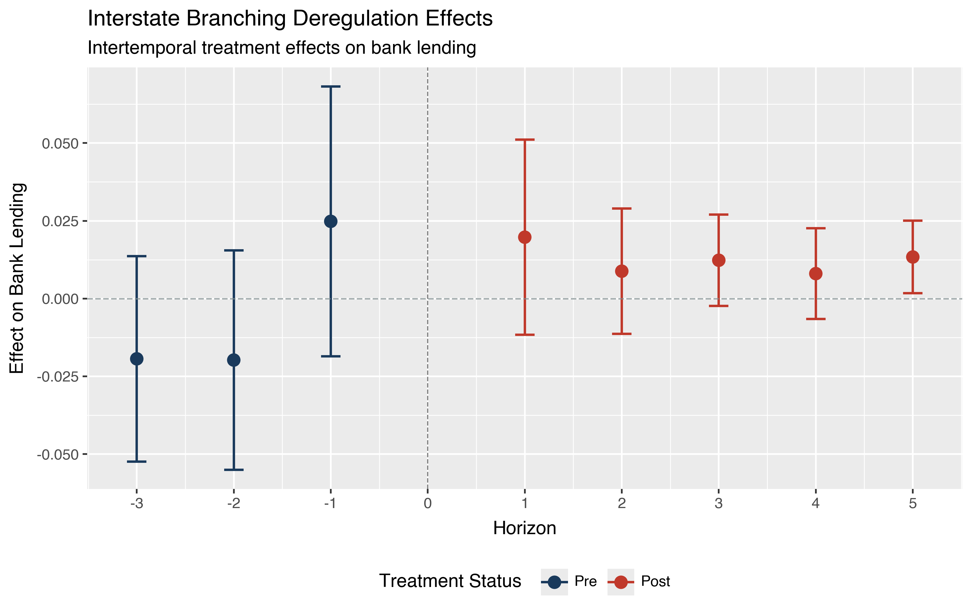
The blue points at negative horizons are pre-treatment placebos. They cluster around zero, consistent with parallel trends. The red points at positive horizons show treatment effects that are positive and relatively stable over time after normalization.
Restricting the comparison#
By default, did_multiplegt pools all units whose treatment changed,
regardless of the direction of the change. Setting switchers="in"
restricts estimation to units whose treatment increased, while
switchers="out" restricts to units whose treatment decreased. This is
useful for checking whether effects are driven by one direction of change or
for settings where treatment increases and decreases have qualitatively
different implications.
result_in = md.did_multiplegt(
    data=df,
    yname="Dl_vloans_b",
    idname="county",
    tname="year",
    dname="inter_bra",
    effects=5,
    cluster="state_n",
    switchers="in",
)
In this dataset, deregulation is one-directional (states lifted restrictions
but did not reimpose them), so switchers="in" produces the same results
as the default. In other applications where treatment can increase or
decrease, filtering by direction can reveal asymmetries in the treatment
response.
You can also choose which units form the control group. By default, the
comparison uses not-yet-switchers, which maximizes sample
size but may introduce bias if treatment timing is anticipated. Setting
only_never_switchers=True restricts the control group to units that
never change treatment, giving a cleaner comparison at the cost of fewer
controls.
result_never = md.did_multiplegt(
    data=df,
    yname="Dl_vloans_b",
    idname="county",
    tname="year",
    dname="inter_bra",
    effects=5,
    cluster="state_n",
    only_never_switchers=True,
)
With only 129 never-switchers in this dataset, the sample sizes at each horizon drop substantially (from roughly 3,800 to 1,600 at horizon 1) and standard errors increase. The point estimates remain positive and, if anything, are larger than the baseline, suggesting that the main results are not driven by contamination from not-yet-switchers in the control group.
Heterogeneous effects#
The predict_het parameter tests whether treatment effects vary across
subgroups defined by time-invariant covariates. It takes a tuple of
(covariate_list, horizon_list) where the horizons specify which effects to
analyze. Use [-1] to analyze all estimated horizons.
import polars as pl

result_het = md.did_multiplegt(
    data=df,
    yname="Dl_vloans_b",
    idname="county",
    tname="year",
    dname="inter_bra",
    effects=3,
    cluster="state_n",
    predict_het=(["state_n"], [-1]),
)

frames = [md.to_df(h) for h in result_het.heterogeneity]
print(pl.concat(frames))
shape: (3, 9)
┌─────────┬───────────┬───────────┬───────────┬───────────┬───────────┬──────────┬─────┬───────────┐
│ Horizon ┆ Covariate ┆ Estimate  ┆ Std.      ┆ t-stat    ┆ CI Lower  ┆ CI Upper ┆ N   ┆ F p-value │
│ ---     ┆ ---       ┆ ---       ┆ Error     ┆ ---       ┆ ---       ┆ ---      ┆ --- ┆ ---       │
│ i64     ┆ str       ┆ f64       ┆ ---       ┆ f64       ┆ f64       ┆ f64      ┆ i64 ┆ f64       │
│         ┆           ┆           ┆ f64       ┆           ┆           ┆          ┆     ┆           │
╞═════════╪═══════════╪═══════════╪═══════════╪═══════════╪═══════════╪══════════╪═════╪═══════════╡
│ 1       ┆ state_n   ┆ -0.001856 ┆ 0.001439  ┆ -1.289654 ┆ -0.00468  ┆ 0.000968 ┆ 904 ┆ 0.197503  │
│ 2       ┆ state_n   ┆ -0.001427 ┆ 0.001249  ┆ -1.142576 ┆ -0.003877 ┆ 0.001024 ┆ 904 ┆ 0.25352   │
│ 3       ┆ state_n   ┆ 0.000174  ┆ 0.001323  ┆ 0.131911  ┆ -0.002421 ┆ 0.00277  ┆ 904 ┆ 0.895084  │
└─────────┴───────────┴───────────┴───────────┴───────────┴───────────┴──────────┴─────┴───────────┘
Under the hood, predict_het regresses each switcher’s signed outcome
change on the specified covariates and cohort fixed effects at each horizon. The F p-value column tests whether the
covariate has any predictive power for treatment effect heterogeneity. Here
the p-values at all three horizons are large (0.20, 0.25, and 0.90),
indicating no evidence that the effect of deregulation on lending varies
systematically across states. For small-sample settings, set
predict_het_hc2bm=True to use Bell-McCaffrey degrees-of-freedom adjusted
standard errors.
Inference options#
By default did_multiplegt computes analytical standard errors using the
influence function. The less_conservative_se and boot parameters
provide two alternatives.
Setting less_conservative_se=True adjusts variance estimation using the
number of distinct (cohort, control-group) cells rather than the total number
of clusters. This typically produces smaller standard errors and is
appropriate when the number of distinct comparison groups is large relative to
the number of clusters.
result_lc = md.did_multiplegt(
    data=df,
    yname="Dl_vloans_b",
    idname="county",
    tname="year",
    dname="inter_bra",
    effects=5,
    cluster="state_n",
    less_conservative_se=True,
)
Setting boot=True uses the multiplier bootstrap for inference instead of
the asymptotic influence function. This is recommended when continuous > 0
(since asymptotic normality is not proven for continuous treatments) and as a
robustness check in small samples. Set biters for the number of
replications and random_state for reproducibility.
result_boot = md.did_multiplegt(
    data=df,
    yname="Dl_vloans_b",
    idname="county",
    tname="year",
    dname="inter_bra",
    effects=3,
    cluster="state_n",
    boot=True,
    biters=999,
    random_state=42,
)
Next steps#
For the complete parameter reference including covariates (controls),
non-parametric trends (trends_nonparam), and confidence level
(ci_level), see the
Intertemporal DiD API reference.
For theoretical background on the de Chaisemartin and D’Haultfoeuille estimator, see the Background section.
For related methods, see the Staggered DiD walkthrough for absorbing treatments and the Continuous DiD walkthrough for another approach to non-binary treatments.