Triple Difference-in-Differences#
Some policies create a natural within-group comparison. A parental leave mandate affects women but not men. A minimum wage increase hits hourly workers but not salaried employees. An education reform applies to public schools but not private ones.
Triple difference-in-differences (DDD) exploits this structure. Beyond comparing treated and control groups before and after policy change, it adds a third comparison between eligible and ineligible subgroups within each group. This additional dimension of variation strengthens causal identification when parallel trends across groups alone might not hold.
The Ortiz-Villavicencio and Sant’Anna (2025) estimator provides doubly robust inference for DDD designs, supporting both two-period and staggered adoption settings.
See also
Introduction to DiD for background on the parallel trends assumption and potential outcomes framework, and Triple Difference-in-Differences for the theoretical foundations behind this estimator.
Three dimensions of variation#
DDD exploits variation along three dimensions simultaneously.
Treatment status distinguishes groups where treatment is enabled (such as
states that pass a policy) from control groups (states that do not). In the
data, this is encoded in the group variable gname.
Eligibility distinguishes units within groups who are affected by the
policy from those who are not. A parental leave policy affects women but not
men. A minimum wage increase affects hourly workers but not salaried employees.
This partition is encoded in the pname variable, where 1 indicates eligible
units and 0 indicates ineligible units.
Time distinguishes pre-treatment from post-treatment periods, as in standard DiD. This creates four subgroups whose outcome changes we can compare.
Treated and eligible units receive the actual treatment
Treated but ineligible units are in treated groups but unaffected
Eligible but untreated units would be affected if their group were treated
Untreated and ineligible units are controls on both dimensions
The DDD estimator computes treatment effects by differencing out trends that are common across groups or across eligibility status, isolating the effect of treatment on eligible units in treated groups.
For a detailed discussion of the identifying assumptions, why standard three-way fixed effects regressions can fail with covariates, and other methodological considerations, see the Background section.
Empirical application#
This example replicates the empirical analysis from Ortiz-Villavicencio and Sant’Anna (2025), which revisits Cai (2016).
In 2003, the People’s Insurance Company of China (PICC) introduced a weather-indexed crop insurance program for tobacco farmers in select counties of Jiangxi province. The program was rolled out in specific treatment regions while other counties served as controls. Within each region, tobacco-growing households were eligible for the insurance while non-tobacco households were not. This creates the three dimensions of variation needed for DDD: treatment region (county 3 vs others), household eligibility (tobacco vs non-tobacco farmers), and time (pre/post 2003).
The outcome of interest is the flexible-term saving ratio
(checksaving_ratio), which measures the share of household income allocated
to liquid savings. The hypothesis is that access to crop insurance reduces
income risk, allowing households to shift savings toward more productive but
less liquid investments. We follow Ortiz-Villavicencio and Sant’Anna (2025) in
using the doubly robust DDD estimator with household-level covariates.
Loading the data#
The dataset is included with ModernDiD and contains 3,659 households observed from 2000 to 2008. The panel is unbalanced, with most households appearing in all 9 years, but some have fewer observations.
import moderndid as did

df = did.load_cai2016()
print(df.shape)
print(df.head(6))
(32391, 10)
shape: (6, 10)
┌──────┬──────┬───────────┬────────┬───┬────────┬──────┬────────────┬────────┐
│ hhno ┆ year ┆ treatment ┆ sector ┆ … ┆ hhsize ┆ age  ┆ educ_scale ┆ county │
│ ---  ┆ ---  ┆ ---       ┆ ---    ┆   ┆ ---    ┆ ---  ┆ ---        ┆ ---    │
│ i64  ┆ i64  ┆ i64       ┆ i64    ┆   ┆ f64    ┆ f64  ┆ f64        ┆ i64    │
╞══════╪══════╪═══════════╪════════╪═══╪════════╪══════╪════════════╪════════╡
│ 1    ┆ 2000 ┆ 1         ┆ 1      ┆ … ┆ 4.0    ┆ 44.0 ┆ 2.0        ┆ 3      │
│ 1    ┆ 2001 ┆ 1         ┆ 1      ┆ … ┆ 4.0    ┆ 45.0 ┆ 2.0        ┆ 3      │
│ 1    ┆ 2002 ┆ 1         ┆ 1      ┆ … ┆ 4.0    ┆ 46.0 ┆ 2.0        ┆ 3      │
│ 1    ┆ 2003 ┆ 1         ┆ 1      ┆ … ┆ 4.0    ┆ 47.0 ┆ 2.0        ┆ 3      │
│ 1    ┆ 2004 ┆ 1         ┆ 1      ┆ … ┆ 4.0    ┆ 48.0 ┆ 2.0        ┆ 3      │
│ 1    ┆ 2005 ┆ 1         ┆ 1      ┆ … ┆ 4.0    ┆ 49.0 ┆ 2.0        ┆ 3      │
└──────┴──────┴───────────┴────────┴───┴────────┴──────┴────────────┴────────┘
Data preparation#
The treatment variable indicates whether a household is in the treatment
region (county 3). Because this indicator is static (it equals 1 in every
period for treated households), we pass treat_period=2003 to
get_group so that treated units are assigned G = 2003 and
controls receive G = 0. We then rename the column to group.
df = did.get_group(df, idname="hhno", tname="year",
                   treatname="treatment", treat_period=2003)
df = df.rename({"G": "group"})

# Subgroup counts (one row per household)
unit_info = df.sort(["hhno", "year"]).group_by("hhno", maintain_order=True).first()
print(
    unit_info.group_by(["treatment", "sector"])
    .len()
    .sort(["treatment", "sector"])
)
shape: (4, 3)
┌───────────┬────────┬──────┐
│ treatment ┆ sector ┆ len  │
│ ---       ┆ ---    ┆ ---  │
│ i64       ┆ i64    ┆ u32  │
╞═══════════╪════════╪══════╡
│ 0         ┆ 0      ┆ 1390 │
│ 0         ┆ 1      ┆ 1271 │
│ 1         ┆ 0      ┆ 161  │
│ 1         ┆ 1      ┆ 837  │
└───────────┴────────┴──────┘
The four subgroups are 1,390 untreated non-tobacco households, 1,271 untreated tobacco households, 161 treated non-tobacco households, and 837 treated tobacco households (the group that actually receives insurance).
Estimation#
We estimate group-time treatment effects using the doubly robust DDD estimator
with household size and age as covariates, following the specification in
Ortiz-Villavicencio and Sant’Anna (2025, Figure 5). Setting
allow_unbalanced_panel=True keeps the estimation in panel mode while
handling households that appear in different subsets of years, preserving
panel-efficient standard errors. We use 999 bootstrap repetitions for
inference.
result = did.ddd(
    data=df,
    yname="checksaving_ratio",
    tname="year",
    idname="hhno",
    gname="group",
    pname="sector",
    xformla="~ hhsize + age",
    control_group="nevertreated",
    base_period="universal",
    est_method="dr",
    allow_unbalanced_panel=True,
    boot=True,
    biters=999,
    random_state=7,
)

event_study = did.agg_ddd(
    result, type="eventstudy", biters=999, cband=False, random_state=7
)
print(event_study)
==============================================================================
 Aggregate DDD Treatment Effects (Event Study)
==============================================================================

 Overall summary of ATT's based on event-study aggregation:

┌────────┬────────────┬────────────────────────┐
│    ATT │ Std. Error │ [95% Conf. Interval]   │
├────────┼────────────┼────────────────────────┤
│ 0.0548 │     0.0137 │ [  0.0278,   0.0817] * │
└────────┴────────────┴────────────────────────┘


 Dynamic Effects:

┌────────────┬──────────┬────────────┬────────────────────────────┐
│ Event time │ Estimate │ Std. Error │ [95% Pointwise Conf. Band] │
├────────────┼──────────┼────────────┼────────────────────────────┤
│         -3 │  -0.0545 │     0.0197 │ [-0.0931, -0.0158] *       │
│         -2 │  -0.0321 │     0.0203 │ [-0.0720,  0.0077]         │
│         -1 │   0.0000 │         NA │ NA                         │
│          0 │   0.0070 │     0.0205 │ [-0.0332,  0.0471]         │
│          1 │   0.0317 │     0.0199 │ [-0.0072,  0.0706]         │
│          2 │   0.0484 │     0.0247 │ [ 0.0000,  0.0967] *       │
│          3 │   0.0422 │     0.0205 │ [ 0.0019,  0.0825] *       │
│          4 │   0.0684 │     0.0262 │ [ 0.0171,  0.1197] *       │
│          5 │   0.1309 │     0.0234 │ [ 0.0851,  0.1767] *       │
└────────────┴──────────┴────────────┴────────────────────────────┘

------------------------------------------------------------------------------
 Signif. codes: '*' confidence band does not cover 0

------------------------------------------------------------------------------
 Data Info
------------------------------------------------------------------------------
 Panel Data
 Outcome variable: checksaving_ratio
 Qualification variable: sector
 Control group: Never Treated
 Base period: universal

------------------------------------------------------------------------------
 Estimation Details
------------------------------------------------------------------------------
 Outcome regression: OLS
 Propensity score: Logistic regression (MLE)

------------------------------------------------------------------------------
 Inference
------------------------------------------------------------------------------
 Significance level: 0.05
 Bootstrap standard errors
==============================================================================
 See Ortiz-Villavicencio and Sant'Anna (2025) for details.
Comparing with three-way fixed effects#
Ortiz-Villavicencio and Sant’Anna (2025) compare their DR-DDD estimator against the standard three-way fixed effects (3WFE) event study specification from Cai (2016, Equation 6.1)
where \(\gamma_i\) are household fixed effects, \(\gamma_{r,t}\) are county-by-year fixed effects, \(\gamma_{j,t}\) are sector-by-year fixed effects, and \(E_{i,t} = t - G_i\) is the event time for treated eligible households. We estimate this using pyfixest.
import numpy as np
import pyfixest as pf

pdf = df.to_pandas()
pdf["rel_time"] = np.where(
    (pdf["treatment"] == 1) & (pdf["sector"] == 1),
    pdf["year"] - 2003,
    -99,
)

fit = pf.feols(
    "checksaving_ratio ~ i(rel_time, ref=-1) + hhsize + age"
    " | hhno + county^year + sector^year",
    data=pdf,
    vcov={"CRV1": "hhno"},
)
Both estimators yield similar point estimates, but the DR-DDD produces tighter confidence intervals at later event times. We overlay the two sets of estimates following the presentation in Ortiz-Villavicencio and Sant’Anna (2025, Figure 5 Panel C).
import pandas as pd

# DR-DDD estimates (to_df() drops the reference period automatically)
drddd_df = did.to_df(event_study).to_pandas()
drddd_df["estimator"] = "DR-DDD"

# 3WFE estimates from pyfixest
tidy = fit.tidy()
rel_coefs = tidy[tidy.index.str.contains("rel_time") & ~tidy.index.str.contains("-99")]
event_times = rel_coefs.index.to_series().str.extract(r"T\.(-?\d+)")[0].astype(int)
twfe_df = pd.DataFrame({
    "event_time": event_times.values,
    "att": rel_coefs["Estimate"].values,
    "ci_lower": rel_coefs["2.5%"].values,
    "ci_upper": rel_coefs["97.5%"].values,
    "estimator": "3WFE",
})

# Combine and restrict to event times >= -2 (Figure 5 window)
plot_df = pd.concat([drddd_df, twfe_df], ignore_index=True)
plot_df = plot_df[plot_df["event_time"] >= -2]

# DR-DDD overall effect for annotation
es_avg = event_study.overall_att
es_lci = es_avg - event_study.crit_val * event_study.overall_se
es_uci = es_avg + event_study.crit_val * event_study.overall_se
Now we can plot.
from plotnine import (
    aes, annotate, element_text, geom_errorbar, geom_hline,
    geom_point, geom_vline, ggplot, labs, position_dodge,
    scale_color_manual, scale_shape_manual, scale_x_continuous,
    theme, theme_gray,
)

caption = """\
3WFE estimates Cai (2016, Eq. 6.1) with household, county-by-year,
and sector-by-year fixed effects. DR-DDD uses the doubly robust
estimator of Ortiz-Villavicencio and Sant'Anna (2025).\
"""

dodge = position_dodge(width=0.25)

p = (
    ggplot(plot_df, aes(x="event_time", y="att", color="estimator",
                        shape="estimator"))
    + geom_hline(yintercept=0, color="black", size=0.4)
    + geom_vline(xintercept=-1, linetype="dashed", color="gray", size=0.4)
    + geom_errorbar(
        aes(ymin="ci_lower", ymax="ci_upper"),
        width=0.15, size=0.6, position=dodge,
    )
    + geom_point(size=3, position=dodge)
    + scale_color_manual(values={"3WFE": "#1a3a5c", "DR-DDD": "#c0392b"})
    + scale_shape_manual(values={"3WFE": "o", "DR-DDD": "^"})
    + scale_x_continuous(
        breaks=sorted(set(plot_df["event_time"].unique()) | {-1}),
    )
    + annotate(
        "text", x=-0.5, y=plot_df["ci_upper"].max() * 0.95,
        label=(f"$\\widehat{{ES}}_{{avg}}$"
               f" = {es_avg:.3f}  [{es_lci:.3f}, {es_uci:.3f}]"),
        ha="left", va="top", size=9,
    )
    + labs(
        x="Event Time",
        y="Treatment Effect (Saving Rate)",
        title="Insurance Provision on Flexible-Term Saving Rate",
        subtitle="Comparing DR-DDD and 3WFE event study estimates"
                 " for Cai (2016) crop insurance data",
        caption=caption,
        color="", shape="",
    )
    + theme_gray()
    + theme(
        legend_position="right",
        plot_caption=element_text(
            ha="left",
            margin={"t": 1, "units": "lines"},
            linespacing=1.25,
        ),
    )
)
p.save("plot_ddd_cai_event_study.png", dpi=200, width=8, height=4.5)
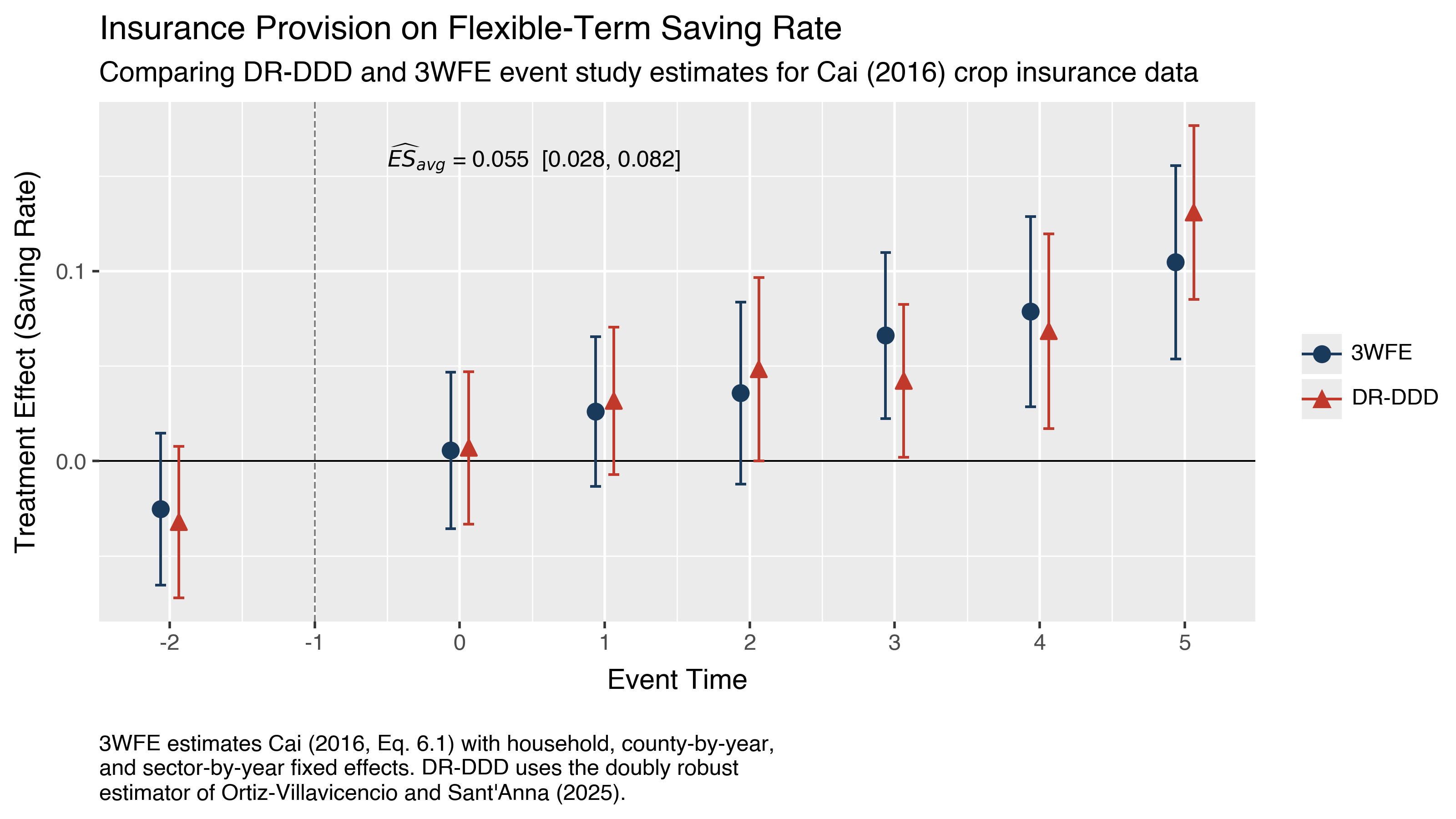
The figure restricts the pre-treatment window to event times \(-2\) and \(-1\) to match the presentation in Ortiz-Villavicencio and Sant’Anna (2025, Figure 5). Both pre-treatment estimates are close to zero and statistically insignificant, supporting the DDD parallel trends assumption. The post-treatment estimates show a gradually increasing pattern, with the effect on the flexible-term saving ratio is near zero at the time of insurance introduction (event time 0) and grows to about 0.13 by five years after treatment (event time 5). Event times 2 through 5 are statistically significant under pointwise confidence bands for the DR-DDD estimator.
The DR-DDD average post-treatment effect is \(\widehat{ES}_{avg} = 0.055\) with 95% CI [0.028, 0.082]. The 3WFE confidence intervals are visibly wider at later event times, consistent with the paper’s finding that 3WFE intervals can be up to 1.15 times wider than the DR-DDD intervals for this application. This precision gain arises because the doubly robust estimator correctly integrates over the treated population’s covariate distribution rather than imposing linear covariate adjustments.
Simulating data#
The following examples use simulated panel data with four subgroups: treated eligible, treated ineligible, untreated eligible, and untreated ineligible.
import moderndid as did

dgp = did.gen_ddd_2periods(n=5000, dgp_type=1, random_state=42)
data = dgp["data"]
print(data.head(6))
shape: (6, 10)
┌─────┬───────┬───────────┬──────┬───┬───────────┬───────────┬──────────┬─────────┐
│ id  ┆ state ┆ partition ┆ time ┆ … ┆ cov2      ┆ cov3      ┆ cov4     ┆ cluster │
│ --- ┆ ---   ┆ ---       ┆ ---  ┆   ┆ ---       ┆ ---       ┆ ---      ┆ ---     │
│ i64 ┆ i64   ┆ i64       ┆ i64  ┆   ┆ f64       ┆ f64       ┆ f64      ┆ i64     │
╞═════╪═══════╪═══════════╪══════╪═══╪═══════════╪═══════════╪══════════╪═════════╡
│ 1   ┆ 0     ┆ 1         ┆ 1    ┆ … ┆ -0.20212  ┆ -0.012154 ┆ 0.862487 ┆ 12      │
│ 1   ┆ 0     ┆ 1         ┆ 2    ┆ … ┆ -0.20212  ┆ -0.012154 ┆ 0.862487 ┆ 12      │
│ 2   ┆ 1     ┆ 1         ┆ 1    ┆ … ┆ -0.408526 ┆ -0.916222 ┆ -0.09073 ┆ 5       │
│ 2   ┆ 1     ┆ 1         ┆ 2    ┆ … ┆ -0.408526 ┆ -0.916222 ┆ -0.09073 ┆ 5       │
│ 3   ┆ 0     ┆ 1         ┆ 1    ┆ … ┆ -0.412515 ┆ -1.059306 ┆ 1.064033 ┆ 1       │
│ 3   ┆ 0     ┆ 1         ┆ 2    ┆ … ┆ -0.412515 ┆ -1.059306 ┆ 1.064033 ┆ 1       │
└─────┴───────┴───────────┴──────┴───┴───────────┴───────────┴──────────┴─────────┘
The data has 5,000 units observed across 2 time periods. The state variable
indicates treatment group membership (0 for control, 1 for treated). The
partition variable indicates eligibility (0 for ineligible, 1 for eligible).
This simulation has no true treatment effect, so the DDD estimate should be
close to zero.
Two-period DDD estimation#
With a simple two-period design where all treated units receive treatment at
the same time, the ddd function estimates the average treatment effect on
treated eligible units.
result = did.ddd(
    data=data,
    yname="y",
    tname="time",
    idname="id",
    gname="state",
    pname="partition",
    xformla="~ cov1 + cov2 + cov3 + cov4",
    est_method="dr",
)
print(result)
==============================================================================
 Triple Difference-in-Differences (DDD) Estimation
==============================================================================

 DR-DDD estimation for the ATT:

┌────────┬────────────┬──────────┬────────────────────────┐
│    ATT │ Std. Error │ Pr(>|t|) │ [95% Conf. Interval]   │
├────────┼────────────┼──────────┼────────────────────────┤
│ 0.0229 │     0.0828 │   0.7825 │ [ -0.1394,   0.1851]   │
└────────┴────────────┴──────────┴────────────────────────┘

------------------------------------------------------------------------------
 Signif. codes: '*' confidence interval does not cover 0

------------------------------------------------------------------------------
 Data Info
------------------------------------------------------------------------------
 Panel Data: 2 periods
 Outcome variable: y
 Qualification variable: partition

 No. of units at each subgroup:
   treated-and-eligible: 1235
   treated-but-ineligible: 1246
   eligible-but-untreated: 1291
   untreated-and-ineligible: 1228

------------------------------------------------------------------------------
 Estimation Details
------------------------------------------------------------------------------
 Outcome regression: OLS
 Propensity score: Logistic regression (MLE)

------------------------------------------------------------------------------
 Inference
------------------------------------------------------------------------------
 Significance level: 0.05
 Analytical standard errors
==============================================================================
 See Ortiz-Villavicencio and Sant'Anna (2025) for details.
We get an ATT estimate of 0.023, close to zero as expected, with a confidence interval that comfortably includes zero. The output also reports the number of units in each of the four subgroups, confirming balanced representation across the design.
The est_method="dr" option uses doubly robust estimation, which combines
outcome regression and propensity score weighting. This approach is consistent
if either the outcome model or the propensity score model is correctly
specified, providing robustness against model misspecification.
Staggered treatment adoption#
When treatment adoption is staggered across groups (some groups adopt in period 2, others in period 3, etc.), we can estimate group-time average treatment effects for each combination of treatment cohort and time period.
dgp_mp = did.gen_ddd_mult_periods(n=500, dgp_type=1, random_state=42)
data_mp = dgp_mp["data"]
print(data_mp.head(6))
shape: (6, 10)
┌─────┬───────┬───────────┬──────┬───┬──────────┬───────────┬───────────┬─────────┐
│ id  ┆ group ┆ partition ┆ time ┆ … ┆ cov2     ┆ cov3      ┆ cov4      ┆ cluster │
│ --- ┆ ---   ┆ ---       ┆ ---  ┆   ┆ ---      ┆ ---       ┆ ---       ┆ ---     │
│ i64 ┆ i64   ┆ i64       ┆ i64  ┆   ┆ f64      ┆ f64       ┆ f64       ┆ i64     │
╞═════╪═══════╪═══════════╪══════╪═══╪══════════╪═══════════╪═══════════╪═════════╡
│ 1   ┆ 2     ┆ 1         ┆ 1    ┆ … ┆ 1.068661 ┆ -0.081955 ┆ -0.218837 ┆ 14      │
│ 1   ┆ 2     ┆ 1         ┆ 2    ┆ … ┆ 1.068661 ┆ -0.081955 ┆ -0.218837 ┆ 14      │
│ 1   ┆ 2     ┆ 1         ┆ 3    ┆ … ┆ 1.068661 ┆ -0.081955 ┆ -0.218837 ┆ 14      │
│ 2   ┆ 3     ┆ 1         ┆ 1    ┆ … ┆ 1.221115 ┆ 0.709174  ┆ -1.161969 ┆ 17      │
│ 2   ┆ 3     ┆ 1         ┆ 2    ┆ … ┆ 1.221115 ┆ 0.709174  ┆ -1.161969 ┆ 17      │
│ 2   ┆ 3     ┆ 1         ┆ 3    ┆ … ┆ 1.221115 ┆ 0.709174  ┆ -1.161969 ┆ 17      │
└─────┴───────┴───────────┴──────┴───┴──────────┴───────────┴───────────┴─────────┘
In multi-period data, the group variable indicates when treatment is first
enabled for each unit (0 for never-treated, 2 for treated starting in period 2,
etc.). This simulation has positive treatment effects that grow over time.
result_mp = did.ddd(
    data=data_mp,
    yname="y",
    tname="time",
    idname="id",
    gname="group",
    pname="partition",
    xformla="~ cov1 + cov2 + cov3 + cov4",
    control_group="nevertreated",
    base_period="universal",
    est_method="dr",
)
print(result_mp)
==============================================================================
 Triple Difference-in-Differences (DDD) Estimation
 Multi-Period / Staggered Treatment Adoption
==============================================================================

 DR-DDD estimation for ATT(g,t):

┌───────┬──────┬──────────┬────────────┬──────────────────────┐
│ Group │ Time │ ATT(g,t) │ Std. Error │ [95% Conf. Int.]     │
├───────┼──────┼──────────┼────────────┼──────────────────────┤
│     2 │    1 │   0.0000 │         NA │ NA                   │
│     2 │    2 │  11.1769 │     0.4201 │ [10.3535, 12.0004] * │
│     2 │    3 │  21.1660 │     0.4516 │ [20.2808, 22.0511] * │
│     3 │    1 │  -1.0095 │     0.5450 │ [-2.0778,  0.0587]   │
│     3 │    2 │   0.0000 │         NA │ NA                   │
│     3 │    3 │  24.9440 │     0.4724 │ [24.0182, 25.8698] * │
└───────┴──────┴──────────┴────────────┴──────────────────────┘

------------------------------------------------------------------------------
 Signif. codes: '*' confidence interval does not cover 0

------------------------------------------------------------------------------
 Data Info
------------------------------------------------------------------------------
 Panel Data
 Outcome variable: y
 Qualification variable: partition
 Control group: Never Treated
 Base period: universal

 No. of units per treatment group:
   Units never enabling treatment: 97
   Units enabling treatment at period 2: 173
   Units enabling treatment at period 3: 230

------------------------------------------------------------------------------
 Estimation Details
------------------------------------------------------------------------------
 Outcome regression: OLS
 Propensity score: Logistic regression (MLE)

------------------------------------------------------------------------------
 Inference
------------------------------------------------------------------------------
 Significance level: 0.05
 Analytical standard errors
==============================================================================
 See Ortiz-Villavicencio and Sant'Anna (2025) for details.
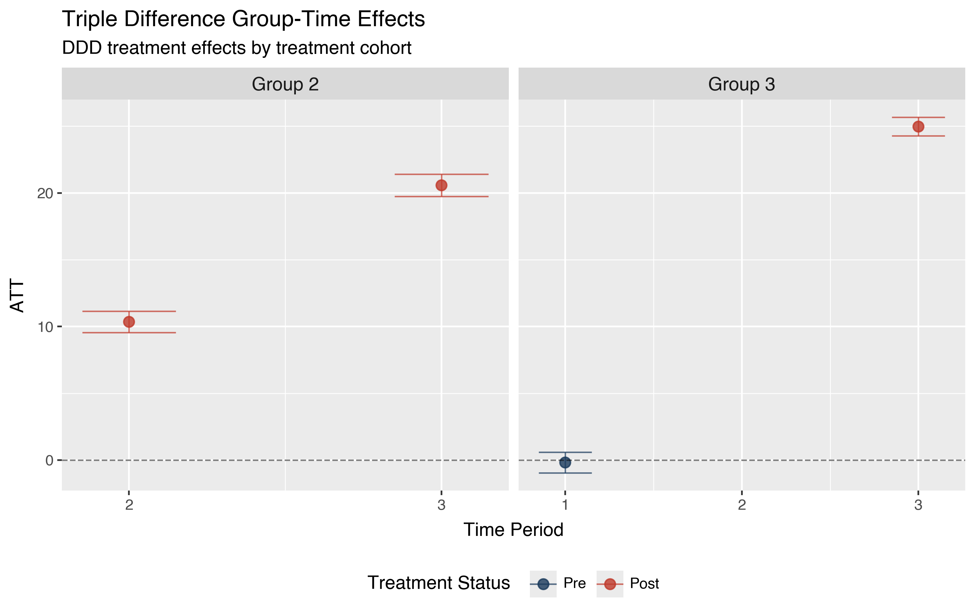
Each row shows the ATT for a specific cohort at a specific time. Rows where Time is before the Group’s treatment date (like Group 2, Time 1) serve as placebo tests. These pre-treatment estimates should be close to zero if the DDD parallel trends assumption is plausible. The estimate of -1.0095 for Group 3 at Time 1 is small relative to the post-treatment effects and statistically insignificant, consistent with the DDD parallel trends assumption.
The post-treatment effects are large and precisely estimated. Group 2 shows effects of 11.2 at time 2 growing to 21.2 at time 3, while Group 3 shows an effect of 24.9 at time 3. The growth from period to period for Group 2 suggests that treatment effects accumulate rather than appearing all at once. Group 3’s larger single-period effect (24.9 vs 11.2 for Group 2 at on-impact) reflects the different treatment effect magnitudes built into the simulation. In applied work, such heterogeneity could arise from differences in cohort composition or treatment intensity across groups.
Aggregating into an event study#
With multiple group-time estimates, there is a lot to digest. The event study aggregation aligns all cohorts relative to their treatment date, making it much easier to see the overall pattern.
event_study = did.agg_ddd(result_mp, type="eventstudy")
print(event_study)
==============================================================================
 Aggregate DDD Treatment Effects (Event Study)
==============================================================================

 Overall summary of ATT's based on event-study aggregation:

┌─────────┬────────────┬────────────────────────┐
│     ATT │ Std. Error │ [95% Conf. Interval]   │
├─────────┼────────────┼────────────────────────┤
│ 20.1000 │     0.3197 │ [ 19.4735,  20.7265] * │
└─────────┴────────────┴────────────────────────┘


 Dynamic Effects:

┌────────────┬──────────┬────────────┬──────────────────────────┐
│ Event time │ Estimate │ Std. Error │ [95% Simult. Conf. Band] │
├────────────┼──────────┼────────────┼──────────────────────────┤
│         -2 │  -1.0095 │     0.5477 │ [-2.3043,  0.2853]       │
│         -1 │   0.0000 │         NA │ NA                       │
│          0 │  19.0341 │     0.2465 │ [18.4514, 19.6167] *     │
│          1 │  21.1660 │     0.4387 │ [20.1288, 22.2031] *     │
└────────────┴──────────┴────────────┴──────────────────────────┘

------------------------------------------------------------------------------
 Signif. codes: '*' confidence band does not cover 0

------------------------------------------------------------------------------
 Data Info
------------------------------------------------------------------------------
 Panel Data
 Outcome variable: y
 Qualification variable: partition
 Control group: Never Treated
 Base period: universal

------------------------------------------------------------------------------
 Estimation Details
------------------------------------------------------------------------------
 Outcome regression: OLS
 Propensity score: Logistic regression (MLE)

------------------------------------------------------------------------------
 Inference
------------------------------------------------------------------------------
 Significance level: 0.05
 Bootstrap standard errors
==============================================================================
 See Ortiz-Villavicencio and Sant'Anna (2025) for details.
Event time 0 is the period of treatment adoption. The pre-treatment estimate at event time -2 is -1.0 and statistically insignificant, consistent with the parallel trends assumption. The on-impact effect at event time 0 is 19.0, growing to 21.2 by event time 1.
Summarizing by cohort#
We can also look at average effects for each treatment cohort, revealing heterogeneity across groups that adopted at different times.
group_agg = did.agg_ddd(result_mp, type="group")
print(group_agg)
==============================================================================
 Aggregate DDD Treatment Effects (Group/Cohort)
==============================================================================

 Overall summary of ATT's based on group/cohort aggregation:

┌─────────┬────────────┬────────────────────────┐
│     ATT │ Std. Error │ [95% Conf. Interval]   │
├─────────┼────────────┼────────────────────────┤
│ 21.1781 │     0.4068 │ [ 20.3808,  21.9754] * │
└─────────┴────────────┴────────────────────────┘


 Group Effects:

┌───────┬──────────┬────────────┬──────────────────────────┐
│ Group │ Estimate │ Std. Error │ [95% Simult. Conf. Band] │
├───────┼──────────┼────────────┼──────────────────────────┤
│     2 │  16.1715 │     0.3780 │ [15.3777, 16.9652] *     │
│     3 │  24.9440 │     0.4641 │ [23.9693, 25.9187] *     │
└───────┴──────────┴────────────┴──────────────────────────┘

------------------------------------------------------------------------------
 Signif. codes: '*' confidence band does not cover 0

------------------------------------------------------------------------------
 Data Info
------------------------------------------------------------------------------
 Panel Data
 Outcome variable: y
 Qualification variable: partition
 Control group: Never Treated
 Base period: universal

------------------------------------------------------------------------------
 Estimation Details
------------------------------------------------------------------------------
 Outcome regression: OLS
 Propensity score: Logistic regression (MLE)

------------------------------------------------------------------------------
 Inference
------------------------------------------------------------------------------
 Significance level: 0.05
 Bootstrap standard errors
==============================================================================
 See Ortiz-Villavicencio and Sant'Anna (2025) for details.
Group 2 (early adopters) shows an average effect of 16.2, while Group 3 (later adopters) shows a larger effect of 24.9. This heterogeneity could reflect different treatment intensities, composition effects, or the fact that later cohorts have fewer post-treatment periods averaged into their estimates.
Overall average effect#
If you need a single summary number, the simple aggregation averages across all post-treatment group-time cells.
simple_agg = did.agg_ddd(result_mp, type="simple")
print(simple_agg)
==============================================================================
 Aggregate DDD Treatment Effects
==============================================================================

 Overall ATT:

┌─────────┬────────────┬────────────────────────┐
│     ATT │ Std. Error │ [95% Conf. Interval]   │
├─────────┼────────────┼────────────────────────┤
│ 19.6744 │     0.3004 │ [ 19.0857,  20.2631] * │
└─────────┴────────────┴────────────────────────┘

------------------------------------------------------------------------------
 Signif. codes: '*' confidence band does not cover 0

------------------------------------------------------------------------------
 Data Info
------------------------------------------------------------------------------
 Panel Data
 Outcome variable: y
 Qualification variable: partition
 Control group: Never Treated
 Base period: universal

------------------------------------------------------------------------------
 Estimation Details
------------------------------------------------------------------------------
 Outcome regression: OLS
 Propensity score: Logistic regression (MLE)

------------------------------------------------------------------------------
 Inference
------------------------------------------------------------------------------
 Significance level: 0.05
 Bootstrap standard errors
==============================================================================
 See Ortiz-Villavicencio and Sant'Anna (2025) for details.
The overall ATT of 19.67 represents the average treatment effect across all treated eligible units in all post-treatment periods, weighted by group size.
Plotting results#
Visualizations make it easier to communicate findings. We can start with the group-time plot showing all underlying estimates organized by cohort.
from plotnine import element_text, labs, theme, theme_gray

p = did.plot_gt(result_mp, ncol=2)
p = (p
    + labs(
        x="Time Period",
        y="ATT",
        title="Triple Difference Group-Time Effects",
        subtitle="DDD treatment effects by treatment cohort",
    )
    + theme_gray()
    + theme(
        legend_position="bottom",
        strip_text=element_text(size=11, weight="bold"),
    )
)
p.save("plot_ddd_gt.png", dpi=200, width=8, height=5)
The event study plot shows effects relative to treatment adoption with confidence bands. The vertical dotted line marks the reference period.
p = did.plot_event_study(event_study, ref_period=-1)
p = (p
    + labs(
        x="Years Relative to Treatment",
        y="ATT",
        title="Triple Difference Event Study",
        subtitle="Aggregated event study from staggered DDD estimation",
    )
    + theme_gray()
    + theme(legend_position="bottom")
)
p.save("plot_ddd_event_study.png", dpi=200, width=8, height=5)
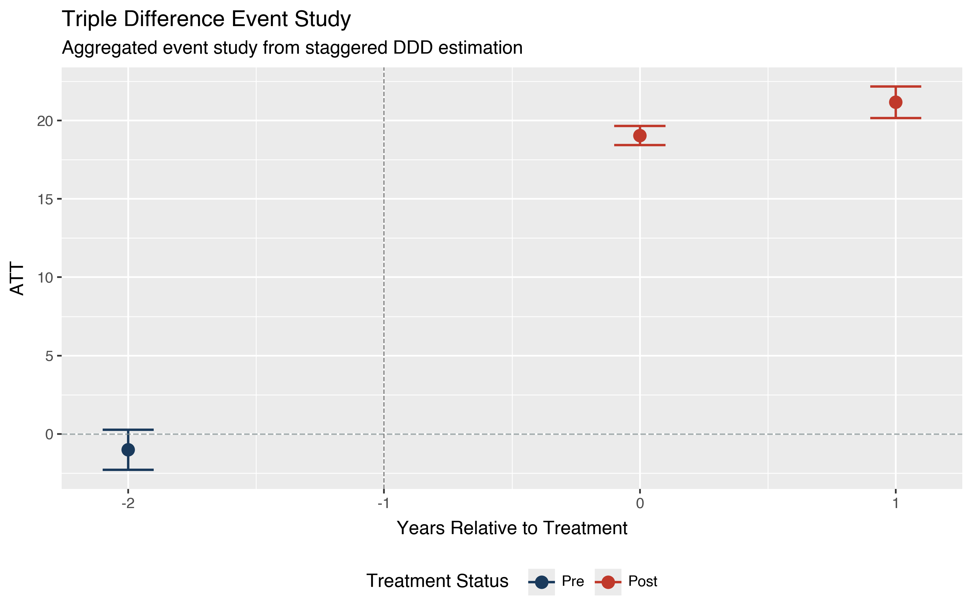
The flat pre-treatment estimate is consistent with the identifying assumptions, though passing pre-treatment placebos alone does not guarantee that the assumption holds in post-treatment periods. The growing post-treatment effects indicate a positive and accumulating treatment effect.
Control group options#
Like the standard staggered DiD estimator, DDD supports different control group definitions.
Never Treated (default) uses only units that never receive treatment during the sample period as controls.
Not Yet Treated uses units that will eventually be treated but have not yet received treatment as additional controls. This can improve efficiency but requires stronger assumptions.
result_nyt = did.ddd(
    data=data_mp,
    yname="y",
    tname="time",
    idname="id",
    gname="group",
    pname="partition",
    xformla="~ cov1 + cov2 + cov3 + cov4",
    control_group="notyettreated",
    base_period="universal",
    est_method="dr",
)
With not-yet-treated controls, some standard errors may be smaller because more observations contribute to the control group comparison.
Repeated cross-section data#
If your data is a repeated cross-section where different units are sampled in
each period, that works too. Just set panel=False.
dgp_rcs = did.gen_ddd_2periods(n=5000, dgp_type=1, panel=False, random_state=42)
data_rcs = dgp_rcs["data"]

result_rcs = did.ddd(
    data=data_rcs,
    yname="y",
    tname="time",
    idname="id",
    gname="state",
    pname="partition",
    xformla="~ cov1 + cov2 + cov3 + cov4",
    est_method="dr",
    panel=False,
)
The estimation method automatically adapts to the repeated cross-section structure, fitting separate outcome models for each subgroup rather than tracking individual units over time.
Next steps#
For details on additional estimation options including bootstrap inference, clustering, and estimation methods, see the Triple DiD API reference.
For theoretical background on triple difference-in-differences, see the Background section.
For the standard two-difference version that this estimator extends, see the Staggered DiD walkthrough.