Sensitivity Analysis for Parallel Trends#
Flat pre-trends are a good sign in any difference-in-differences analysis, but they do not guarantee that parallel trends would have continued after treatment. The identifying assumption is fundamentally untestable.
The Rambachan and Roth (2023) sensitivity analysis reframes the problem. Rather than asking whether parallel trends holds, it asks how large violations would need to be to overturn the conclusions. This approach bounds the magnitude of possible violations and reports confidence intervals that remain valid under those bounds.
This example demonstrates sensitivity analysis using state-level data on health insurance coverage following Medicaid expansion under the Affordable Care Act.
See also
Introduction to DiD for background on the parallel trends assumption and potential outcomes framework, and Honest DiD Sensitivity Analysis for the theoretical foundations behind this estimator.
Why sensitivity analysis matters#
Standard difference-in-differences relies on the assumption that treated and comparison groups would have followed parallel paths absent treatment. When this assumption fails, your estimated treatment effect picks up the difference in trends on top of any real effect.
Pre-trend tests are the most common way to assess this assumption. If the groups were evolving similarly before treatment, it seems plausible they would have continued to do so afterward. But pre-trend tests have well-documented limitations. They may lack statistical power, meaning a failure to reject parallel pre-trends does not mean the assumption actually holds. Your sample may simply be too small or noisy to detect a real divergence.
Sensitivity analysis takes a different approach. Instead of testing whether parallel trends holds exactly, it asks how your conclusions change under different assumptions about the magnitude of violations. If results hold up under plausible violations, you can be more confident in your findings. If results are sensitive, that tells you something important about the fragility of the research design.
Loading data#
import polars as pl
import moderndid as did

data = did.load_ehec()
print(data.head())
shape: (5, 5)
┌────────┬──────┬──────────┬───────┬──────────┐
│ stfips ┆ year ┆ dins     ┆ yexp2 ┆ W        │
│ ---    ┆ ---  ┆ ---      ┆ ---   ┆ ---      │
│ i64    ┆ i64  ┆ f64      ┆ f64   ┆ f64      │
╞════════╪══════╪══════════╪═══════╪══════════╡
│ 1      ┆ 2008 ┆ 0.681412 ┆ null  ┆ 613156.0 │
│ 1      ┆ 2009 ┆ 0.658062 ┆ null  ┆ 613156.0 │
│ 1      ┆ 2010 ┆ 0.631365 ┆ null  ┆ 613156.0 │
│ 1      ┆ 2011 ┆ 0.656389 ┆ null  ┆ 613156.0 │
│ 1      ┆ 2012 ┆ 0.670811 ┆ null  ┆ 613156.0 │
└────────┴──────┴──────────┴───────┴──────────┘
The dataset contains state-level observations from 2008 to 2019. The outcome
dins is the share of adults with health insurance. The yexp2 variable
indicates when each state expanded Medicaid, with null values for states that
never expanded during this period. Some states expanded in 2014 when the ACA
provision took effect, while others expanded later in 2015, 2016, 2017, or 2019.
This staggered adoption pattern is typical of policy evaluations. Different states adopted at different times based on their own political and economic circumstances, which may also affect outcome trends. This is precisely why sensitivity analysis is valuable. Treatment timing may correlate with unobserved factors that also influence outcomes.
Computing the event study#
Sensitivity analysis requires an event study as input. We start by estimating group-time average treatment effects, then aggregate them into an event study that aligns all cohorts relative to their treatment date.
# Handle the treatment timing variable
data = data.with_columns(
    pl.when(pl.col("yexp2").is_null())
    .then(0)
    .otherwise(pl.col("yexp2"))
    .cast(pl.Int64)
    .alias("first_treat")
)

# Estimate group-time effects
gt_result = did.att_gt(
    data=data,
    yname="dins",
    tname="year",
    idname="stfips",
    gname="first_treat",
    control_group="notyettreated",
)

# Aggregate to event study
event_study = did.aggte(gt_result, type="dynamic")
print(event_study)
==============================================================================
 Aggregate Treatment Effects (Event Study)
==============================================================================

 Overall summary of ATT's based on event-study/dynamic aggregation:

┌────────┬────────────┬────────────────────────┐
│    ATT │ Std. Error │ [95% Conf. Interval]   │
├────────┼────────────┼────────────────────────┤
│ 0.0688 │     0.0080 │ [  0.0532,   0.0845] * │
└────────┴────────────┴────────────────────────┘


 Dynamic Effects:

┌────────────┬──────────┬────────────┬────────────────────────────┐
│ Event time │ Estimate │ Std. Error │ [95% Pointwise Conf. Band] │
├────────────┼──────────┼────────────┼────────────────────────────┤
│        -10 │   0.0189 │     0.0050 │ [ 0.0050,  0.0328] *       │
│         -9 │  -0.0269 │     0.0081 │ [-0.0496, -0.0041] *       │
│         -8 │  -0.0129 │     0.0098 │ [-0.0402,  0.0145]         │
│         -7 │  -0.0014 │     0.0075 │ [-0.0223,  0.0195]         │
│         -6 │   0.0189 │     0.0080 │ [-0.0036,  0.0414]         │
│         -5 │  -0.0084 │     0.0051 │ [-0.0226,  0.0059]         │
│         -4 │   0.0054 │     0.0066 │ [-0.0130,  0.0238]         │
│         -3 │   0.0026 │     0.0047 │ [-0.0104,  0.0157]         │
│         -2 │  -0.0012 │     0.0037 │ [-0.0115,  0.0090]         │
│         -1 │   0.0049 │     0.0040 │ [-0.0063,  0.0162]         │
│          0 │   0.0453 │     0.0060 │ [ 0.0284,  0.0621] *       │
│          1 │   0.0651 │     0.0082 │ [ 0.0421,  0.0880] *       │
│          2 │   0.0759 │     0.0084 │ [ 0.0525,  0.0994] *       │
│          3 │   0.0726 │     0.0089 │ [ 0.0478,  0.0974] *       │
│          4 │   0.0738 │     0.0109 │ [ 0.0433,  0.1043] *       │
│          5 │   0.0803 │     0.0103 │ [ 0.0515,  0.1091] *       │
└────────────┴──────────┴────────────┴────────────────────────────┘

------------------------------------------------------------------------------
 Signif. codes: '*' confidence band does not cover 0

------------------------------------------------------------------------------
 Data Info
------------------------------------------------------------------------------
 Control Group: Not Yet Treated
 Anticipation Periods: 0

------------------------------------------------------------------------------
 Estimation Details
------------------------------------------------------------------------------
 Estimation Method: Doubly Robust

------------------------------------------------------------------------------
 Inference
------------------------------------------------------------------------------
 Significance level: 0.05
 Analytical standard errors
==============================================================================
 Reference: Callaway and Sant'Anna (2021)
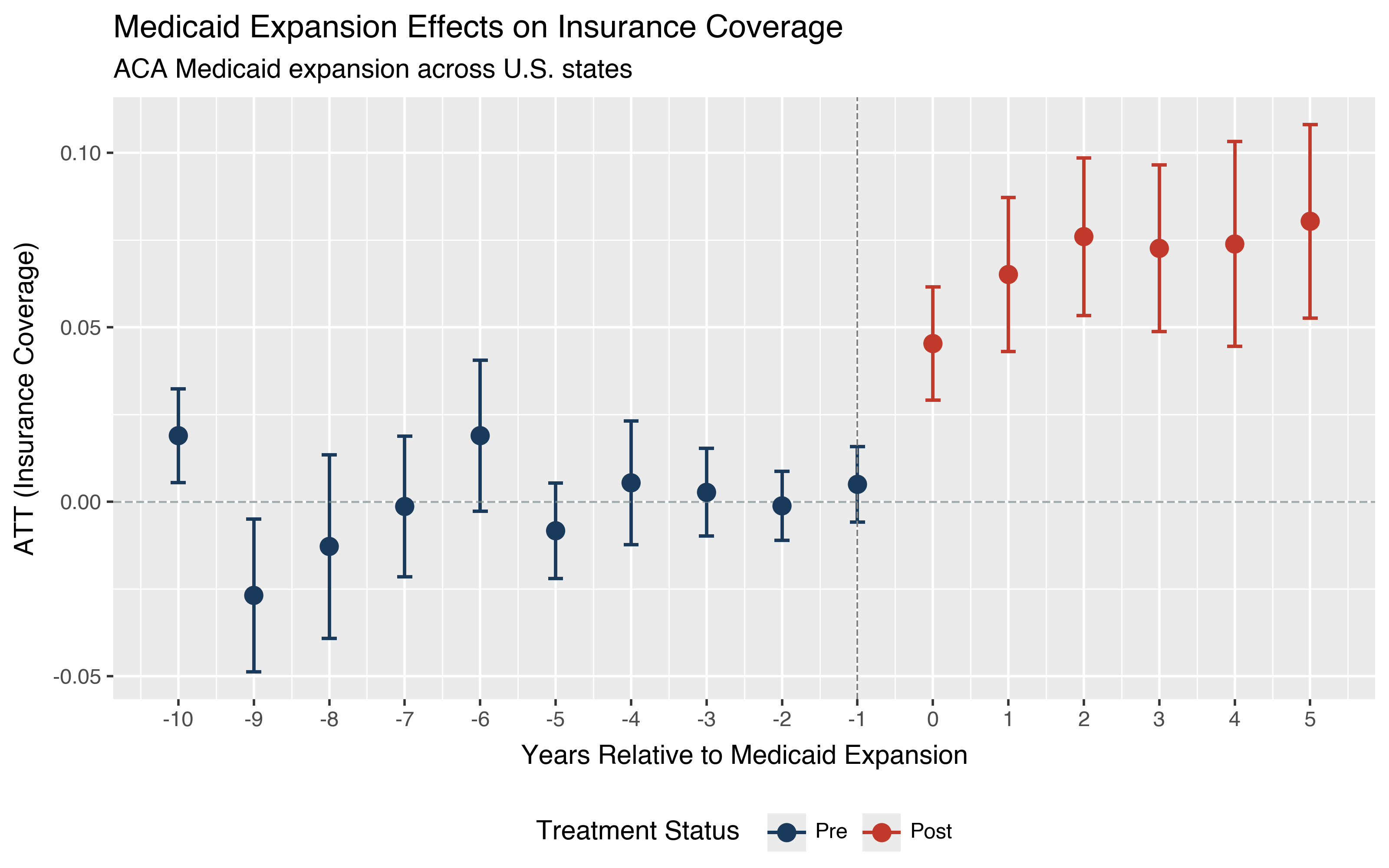
The pre-treatment estimates are mostly close to zero, though there is some variation (a couple of early periods show significance with pointwise bands). The post-treatment estimates show insurance coverage increasing by about 4.5 percentage points on impact, growing to around 8 percentage points five years later. The overall ATT of 0.069 confirms a sizable and statistically significant average effect across all post-treatment periods.
But passing this informal pre-trend test does not prove parallel trends holds. The pre-treatment estimates have confidence intervals that span meaningful violations. Let’s use sensitivity analysis to see how robust these conclusions really are.
from plotnine import labs, theme, theme_gray

p = did.plot_event_study(event_study, ref_period=-1)
p = (p
    + labs(
        x="Years Relative to Medicaid Expansion",
        y="ATT (Insurance Coverage)",
        title="Medicaid Expansion Effects on Insurance Coverage",
        subtitle="ACA Medicaid expansion across U.S. states",
    )
    + theme_gray()
    + theme(legend_position="bottom")
)
p.save("plot_event_study_ehec.png", dpi=200, width=8, height=5)
Smoothness restrictions#
One natural assumption is that violations of parallel trends evolve smoothly over time. If confounding factors are driven by gradual economic or demographic shifts, large sudden changes in the differential trend are implausible. The smoothness restriction bounds how much the slope of the differential trend can change between consecutive periods.
Formally, the smoothness restriction bounds the discrete second derivative of the trend. A bound of M = 0 requires the differential trend to be exactly linear. Larger values of M allow increasingly nonlinear violations. The researcher chooses M based on what magnitude of nonlinearity seems plausible given the economic context.
from moderndid.didhonest import honest_did

# Analyze the on-impact effect (event_time=0)
sensitivity_sm = honest_did(
    event_study=event_study,
    event_time=0,
    sensitivity_type="smoothness",
    m_vec=[0.0, 0.005, 0.01, 0.015, 0.02],
)
print(sensitivity_sm.robust_ci)
shape: (5, 5)
┌──────────┬──────────┬────────┬─────────┬───────┐
│ lb       ┆ ub       ┆ method ┆ delta   ┆ m     │
│ ---      ┆ ---      ┆ ---    ┆ ---     ┆ ---   │
│ f64      ┆ f64      ┆ str    ┆ str     ┆ f64   │
╞══════════╪══════════╪════════╪═════════╪═══════╡
│ 0.022141 ┆ 0.043601 ┆ FLCI   ┆ DeltaSD ┆ 0.0   │
│ 0.028764 ┆ 0.059345 ┆ FLCI   ┆ DeltaSD ┆ 0.005 │
│ 0.023794 ┆ 0.064312 ┆ FLCI   ┆ DeltaSD ┆ 0.01  │
│ 0.018794 ┆ 0.069312 ┆ FLCI   ┆ DeltaSD ┆ 0.015 │
│ 0.013794 ┆ 0.074312 ┆ FLCI   ┆ DeltaSD ┆ 0.02  │
└──────────┴──────────┴────────┴─────────┴───────┘
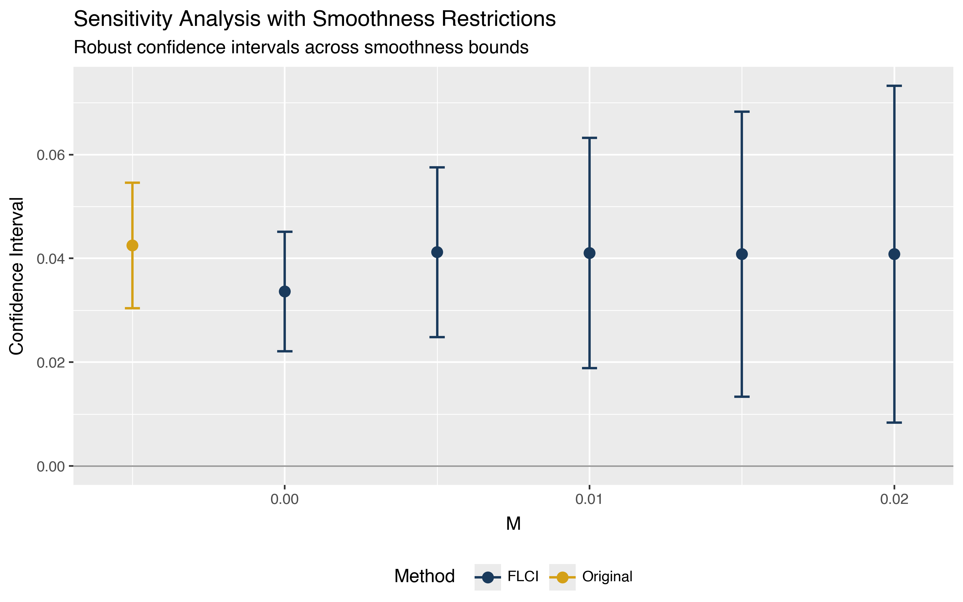
Each row shows a robust confidence interval under a different smoothness bound. When M = 0, the differential trend must be exactly linear. Under this strong assumption, you can rule out zero. The lower bound of the confidence interval is 2.2 percentage points. As M increases and allows more nonlinearity, the confidence intervals widen. Even at M = 0.02, the lower bound remains positive at 1.4 percentage points.
The interpretation depends on what values of M are considered plausible. Given that the pre-treatment estimates show relatively flat trends with small fluctuations, smoothness bounds around 0.01 to 0.02 represent similar magnitudes of nonlinearity. Under these bounds, the evidence for a positive effect remains robust.
The original confidence interval assuming exact parallel trends can be retrieved from the result object.
print(f"Original CI: [{sensitivity_sm.original_ci.lb:.4f}, {sensitivity_sm.original_ci.ub:.4f}]")
Original CI: [0.0335, 0.0571]
The built-in plotting function visualizes how the confidence interval changes with the smoothness bound.
p = did.plot_sensitivity(sensitivity_sm)
p = (p
    + labs(
        title="Sensitivity Analysis with Smoothness Restrictions",
        subtitle="Robust confidence intervals across smoothness bounds",
    )
    + theme_gray()
    + theme(legend_position="bottom")
)
p.save("plot_sensitivity_smoothness.png", dpi=200, width=8, height=5)
Relative magnitudes restrictions#
We can also bound post-treatment violations of parallel trends relative to the maximum pre-treatment violation. Specifically, the restriction applies to period-to-period changes in the differential trend. If the confounding factors that create violations are of similar magnitude before and after treatment, this restriction is natural.
The parameter Mbar controls the bound. When Mbar = 1, the maximum period-to-period violation after treatment cannot exceed the maximum period-to-period violation before treatment. When Mbar = 2, it can be up to twice as large, and so on.
sensitivity_rm = honest_did(
    event_study=event_study,
    event_time=0,
    sensitivity_type="relative_magnitude",
    m_bar_vec=[0.5, 1.0, 1.5, 2.0],
)
print(sensitivity_rm.robust_ci)
shape: (4, 5)
┌───────────┬──────────┬────────┬─────────┬──────┐
│ lb        ┆ ub       ┆ method ┆ delta   ┆ Mbar │
│ ---       ┆ ---      ┆ ---    ┆ ---     ┆ ---  │
│ f64       ┆ f64      ┆ str    ┆ str     ┆ f64  │
╞═══════════╪══════════╪════════╪═════════╪══════╡
│ 0.022173  ┆ 0.073241 ┆ C-LF   ┆ DeltaRM ┆ 0.5  │
│ 0.000287  ┆ 0.092695 ┆ C-LF   ┆ DeltaRM ┆ 1.0  │
│ -0.019168 ┆ 0.114582 ┆ C-LF   ┆ DeltaRM ┆ 1.5  │
│ -0.041054 ┆ 0.136468 ┆ C-LF   ┆ DeltaRM ┆ 2.0  │
└───────────┴──────────┴────────┴─────────┴──────┘
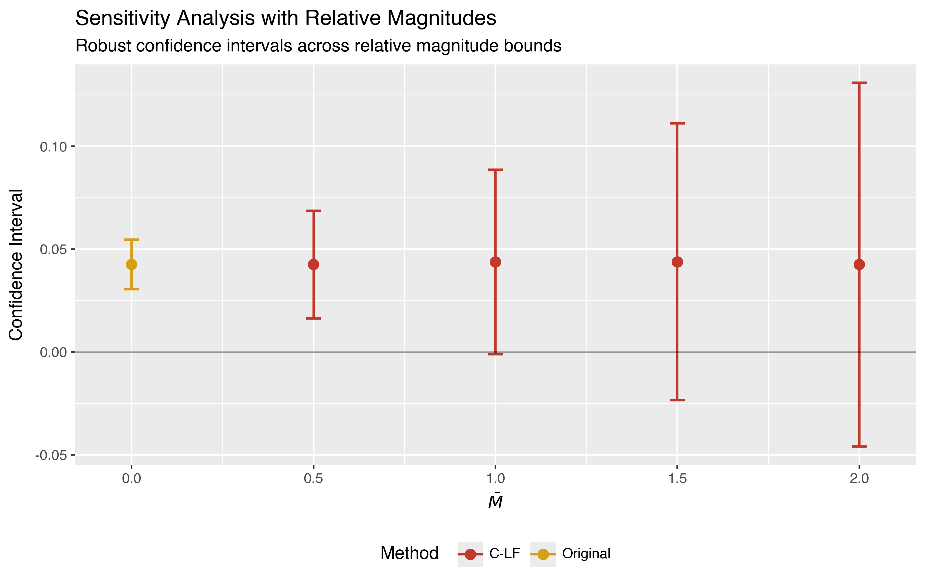
When post-treatment violations are bounded to be at most half the maximum pre-treatment violation (Mbar = 0.5), the confidence interval excludes zero. At Mbar = 1, the benchmark case where violations are bounded by the pre-treatment maximum, the lower bound is barely positive at 0.03 percentage points. By Mbar = 1.5, the confidence interval includes zero.
The method column shows C-LF (conditional-least favorable hybrid)
rather than FLCI. The implementation automatically selects the appropriate
inference method for each restriction type. See the
Background for
details on why different methods are used.
p = did.plot_sensitivity(sensitivity_rm)
p = (p
    + labs(
        title="Sensitivity Analysis with Relative Magnitudes",
        subtitle="Robust confidence intervals across relative magnitude bounds",
    )
    + theme_gray()
    + theme(legend_position="bottom")
)
p.save("plot_sensitivity_rm.png", dpi=200, width=8, height=5)
Analyzing longer-term effects#
We can apply the sensitivity analysis to any post-treatment event time. Effects at longer horizons are often of greater interest for policy evaluation but may also be more susceptible to violations of parallel trends as confounding factors accumulate.
# Analyze the effect 3 years after treatment
sensitivity_t3 = honest_did(
    event_study=event_study,
    event_time=3,
    sensitivity_type="smoothness",
    m_vec=[0.0, 0.005, 0.01, 0.015, 0.02],
)
print(sensitivity_t3.robust_ci)
shape: (5, 5)
┌───────────┬──────────┬────────┬─────────┬───────┐
│ lb        ┆ ub       ┆ method ┆ delta   ┆ m     │
│ ---       ┆ ---      ┆ ---    ┆ ---     ┆ ---   │
│ f64       ┆ f64      ┆ str    ┆ str     ┆ f64   │
╞═══════════╪══════════╪════════╪═════════╪═══════╡
│ 0.051576  ┆ 0.084122 ┆ FLCI   ┆ DeltaSD ┆ 0.0   │
│ 0.002072  ┆ 0.150059 ┆ FLCI   ┆ DeltaSD ┆ 0.005 │
│ -0.058358 ┆ 0.19724  ┆ FLCI   ┆ DeltaSD ┆ 0.01  │
│ -0.110472 ┆ 0.245813 ┆ FLCI   ┆ DeltaSD ┆ 0.015 │
│ -0.160472 ┆ 0.295813 ┆ FLCI   ┆ DeltaSD ┆ 0.02  │
└───────────┴──────────┴────────┴─────────┴───────┘
We see that the three-year effect is larger (around 6.8 percentage points) and remains statistically significant under the assumption of exactly linear trends (M = 0). At M = 0.005, the lower bound is still positive at 0.2 percentage points. By M = 0.01, the confidence interval includes zero. The longer-term effects are more sensitive to violations of parallel trends than the on-impact effect, which makes sense since violations can accumulate over time.
Choosing sensitivity parameters#
Choosing the right values for M (smoothness) or Mbar (relative magnitudes) comes down to judgment about what violations are economically plausible. Rambachan and Roth (2023) offer several helpful guidelines.
For smoothness restrictions, M = 0 corresponds to the parametric assumption of exactly linear differential trends, which is common in applied work. Positive values of M relax this assumption. A natural calibration is to examine the observed nonlinearity in the pre-treatment period. If the pre-treatment estimates fluctuate by at most 0.5 percentage points from a linear trend, then M values up to 0.005 or 0.01 represent similar magnitudes of nonlinearity.
For relative magnitudes restrictions, Mbar = 1 is a natural benchmark. The post-treatment violation is bounded by the maximum pre-treatment violation. Values greater than 1 allow for the possibility that confounding factors are stronger after treatment than before, which may be plausible if the policy itself triggers additional changes.
The goal is not to find a single correct bound, but to show how your conclusions hold up across a range of plausible assumptions. If results are robust to reasonable violations, that strengthens credibility. If results are sensitive, that is valuable information for your readers about the limitations of the analysis.
Incorporating sign restrictions#
Economic knowledge sometimes suggests the direction of potential violations.
If a concurrent policy change would bias estimates upward, the researcher
might impose that violations are positive. The bias_direction parameter
incorporates such restrictions.
sensitivity_pos = honest_did(
    event_study=event_study,
    event_time=0,
    sensitivity_type="smoothness",
    m_vec=[0.0, 0.005, 0.01, 0.015, 0.02],
    bias_direction="positive",
)
When violations are restricted to be positive (upward bias), the upper bound of the confidence interval remains the same as before, but the lower bound may tighten. If the researcher has reason to believe that any confounding would bias estimates upward, this restriction yields more informative confidence intervals for the lower bound of the effect.
Monotonicity restrictions#
In some settings, violations of parallel trends are expected to be
monotone over time. For example, if a secular demographic trend is
the main source of confounding, the bias would gradually increase or
decrease rather than fluctuating. The monotonicity_direction
parameter imposes such restrictions.
sensitivity_inc = honest_did(
    event_study=event_study,
    event_time=0,
    sensitivity_type="smoothness",
    m_vec=[0.0, 0.005, 0.01, 0.015, 0.02],
    monotonicity_direction="increasing",
)
When the differential trend is restricted to be increasing, the confidence intervals may be tighter than under unrestricted smoothness bounds. However, monotonicity is a strong assumption that should be justified by economic reasoning about the specific sources of potential confounding.
Recommendations#
Based on the theoretical results and simulations in Rambachan and Roth (2023), here is what the authors recommend.
Use FLCI for smoothness restrictions. Fixed-length confidence intervals have near-optimal expected length in finite samples when the smoothness bound M is known. The implementation automatically uses this method when
sensitivity_type="smoothness".Use C-LF for relative magnitudes restrictions. FLCIs can be inconsistent under these restrictions because the identified set length depends on the pre-treatment maximum violation. The implementation automatically uses the conditional-least favorable hybrid when
sensitivity_type="relative_magnitude".Report results for a range of violation bounds rather than a single value. This makes clear what must be assumed to draw specific conclusions. If results are robust across all plausible bounds, your findings are on solid ground. If results are sensitive, your readers deserve to know that.
Combine sensitivity analysis with economic reasoning about the sources of potential confounding. The goal is not purely statistical. You want to understand whether violations large enough to overturn your conclusions are actually plausible given the institutional context.
Using external event study estimates#
The examples above use ModernDiD’s att_gt and aggte functions to
compute event study estimates. If you already have event study coefficients
from another estimator (such as pyfixest, statsmodels, or another package),
you can plug them directly into the sensitivity analysis.
The direct API requires two inputs from your external estimation.
betahat - A numpy array of event study coefficients ordered chronologically, with pre-treatment periods first followed by post-treatment periods. The reference period (typically t = -1) should be excluded.
sigma - The variance-covariance matrix for the coefficients in betahat, as a numpy array with shape (
len(betahat),len(betahat)).
With these inputs, use the lower-level functions directly.
from moderndid.didhonest import (
    construct_original_cs,
    create_sensitivity_results_rm,
    create_sensitivity_results_sm,
)

# Construct original confidence interval
original_ci = construct_original_cs(
    betahat=betahat,
    sigma=sigma,
    num_pre_periods=5,  # number of pre-treatment coefficients
    num_post_periods=2,  # number of post-treatment coefficients
    alpha=0.05
)

# Relative magnitudes sensitivity
rm_results = create_sensitivity_results_rm(
    betahat=betahat,
    sigma=sigma,
    num_pre_periods=5,
    num_post_periods=2,
    m_bar_vec=[0.5, 1.0, 1.5, 2.0],
    method="C-LF"
)

# Smoothness sensitivity
sm_results = create_sensitivity_results_sm(
    betahat=betahat,
    sigma=sigma,
    num_pre_periods=5,
    num_post_periods=2,
    m_vec=[0.0, 0.01, 0.02, 0.03],
    method="FLCI"
)
By default, these functions target the first post-treatment period. The
l_vec parameter can be used to analyze different linear combinations
of post-treatment effects. For example, set l_vec=np.array([0.5, 0.5])
to analyze the average of two post-treatment periods.
Next steps#
For details on estimation options and the full API, see the Sensitivity Analysis API reference.
For theoretical background on the sensitivity analysis methodology, see the Background section.
For the staggered DiD estimator whose results this analysis builds on, see the Staggered DiD walkthrough.