Staggered Difference-in-Differences#
In practice, policies often roll out gradually over time. One state raises its minimum wage in 2004, another in 2006, and a third in 2007. This staggered adoption creates a rich panel structure for causal inference, but it also creates problems for conventional regression approaches.
Two-way fixed effects regression is the go-to method for many applied researchers, but it can produce misleading results when treatment effects vary across cohorts or over time. The Callaway and Sant’Anna (2021) estimator addresses this by computing separate treatment effects for each cohort at each time period, then aggregating them into interpretable summaries like event studies.
See also
Introduction to DiD for background on the parallel trends assumption and potential outcomes framework, and DiD with Multiple Time Periods for the theoretical foundations behind this estimator.
Empirical application#
This example replicates the empirical analysis from Callaway and Sant’Anna (2021), which studies the effect of minimum wage increases on teen employment.
From 2001 to 2007, the US federal minimum wage was flat at $5.15 per hour. During this period, some states raised their minimum wage above the federal level while others did not. This variation in timing creates a natural staggered adoption design. States that raised their minimum wage form treatment cohorts defined by the year of the increase, while states that kept the federal minimum serve as a never-treated control group.
The outcome of interest is log county-level teen employment, drawn from the Quarterly Workforce Indicators (QWI). The dataset contains 500 counties observed annually from 2003 to 2007, with treatment cohorts in 2004, 2006, and 2007. The hypothesis is that minimum wage increases reduce teen employment, since teenagers are disproportionately represented among minimum wage workers and their labor demand is relatively elastic.
There are notable differences between treated and untreated counties. Treated counties tend to be in the Midwest, have larger populations (94,000 vs 53,000 on average), and higher median incomes. These compositional differences motivate the use of conditional parallel trends with covariates, as unconditional comparisons may not adequately control for pre-existing differences between groups.
Loading the data#
import moderndid as did

data = did.load_mpdta()
print(data.head())
shape: (5, 6)
┌──────┬────────────┬──────────┬──────────┬─────────────┬───────┐
│ year ┆ countyreal ┆ lpop     ┆ lemp     ┆ first.treat ┆ treat │
│ ---  ┆ ---        ┆ ---      ┆ ---      ┆ ---         ┆ ---   │
│ i64  ┆ i64        ┆ f64      ┆ f64      ┆ i64         ┆ i64   │
╞══════╪════════════╪══════════╪══════════╪═════════════╪═══════╡
│ 2003 ┆ 8001       ┆ 5.896761 ┆ 8.461469 ┆ 2007        ┆ 1     │
│ 2004 ┆ 8001       ┆ 5.896761 ┆ 8.33687  ┆ 2007        ┆ 1     │
│ 2005 ┆ 8001       ┆ 5.896761 ┆ 8.340217 ┆ 2007        ┆ 1     │
│ 2006 ┆ 8001       ┆ 5.896761 ┆ 8.378161 ┆ 2007        ┆ 1     │
│ 2007 ┆ 8001       ┆ 5.896761 ┆ 8.487352 ┆ 2007        ┆ 1     │
└──────┴────────────┴──────────┴──────────┴─────────────┴───────┘
The first.treat variable encodes treatment timing, with 0 indicating
never-treated counties. This is a balanced panel where each county appears
exactly once per year. The estimator can handle unbalanced panels, but
balanced data simplifies interpretation and improves precision.
Estimation#
We start by estimating treatment effects separately for each cohort at each time period. This avoids the negative weighting problem that can bias two-way fixed effects estimates when treatment effects vary across cohorts or over time.
result = did.att_gt(
    data=data,
    yname="lemp",
    tname="year",
    idname="countyreal",
    gname="first.treat",
)
print(result)
==============================================================================
 Group-Time Average Treatment Effects
==============================================================================

┌───────┬──────┬──────────┬────────────┬────────────────────────────┐
│ Group │ Time │ ATT(g,t) │ Std. Error │ [95% Pointwise Conf. Band] │
├───────┼──────┼──────────┼────────────┼────────────────────────────┤
│  2004 │ 2004 │  -0.0105 │     0.0233 │ [-0.0561,  0.0351]         │
│  2004 │ 2005 │  -0.0704 │     0.0310 │ [-0.1312, -0.0097] *       │
│  2004 │ 2006 │  -0.1373 │     0.0364 │ [-0.2087, -0.0658] *       │
│  2004 │ 2007 │  -0.1008 │     0.0344 │ [-0.1682, -0.0335] *       │
│  2006 │ 2004 │   0.0065 │     0.0233 │ [-0.0392,  0.0522]         │
│  2006 │ 2005 │  -0.0028 │     0.0196 │ [-0.0411,  0.0356]         │
│  2006 │ 2006 │  -0.0046 │     0.0178 │ [-0.0394,  0.0302]         │
│  2006 │ 2007 │  -0.0412 │     0.0202 │ [-0.0809, -0.0016] *       │
│  2007 │ 2004 │   0.0305 │     0.0150 │ [ 0.0010,  0.0600] *       │
│  2007 │ 2005 │  -0.0027 │     0.0164 │ [-0.0349,  0.0294]         │
│  2007 │ 2006 │  -0.0311 │     0.0179 │ [-0.0661,  0.0040]         │
│  2007 │ 2007 │  -0.0261 │     0.0167 │ [-0.0587,  0.0066]         │
└───────┴──────┴──────────┴────────────┴────────────────────────────┘

------------------------------------------------------------------------------
 Signif. codes: '*' confidence band does not cover 0

 P-value for pre-test of parallel trends assumption:  0.1681

------------------------------------------------------------------------------
 Data Info
------------------------------------------------------------------------------
 Control Group:  Never Treated
 Anticipation Periods:  0

------------------------------------------------------------------------------
 Estimation Details
------------------------------------------------------------------------------
 Estimation Method:  Doubly Robust

------------------------------------------------------------------------------
 Inference
------------------------------------------------------------------------------
 Significance level: 0.05
 Analytical standard errors
==============================================================================
 Reference: Callaway and Sant'Anna (2021)
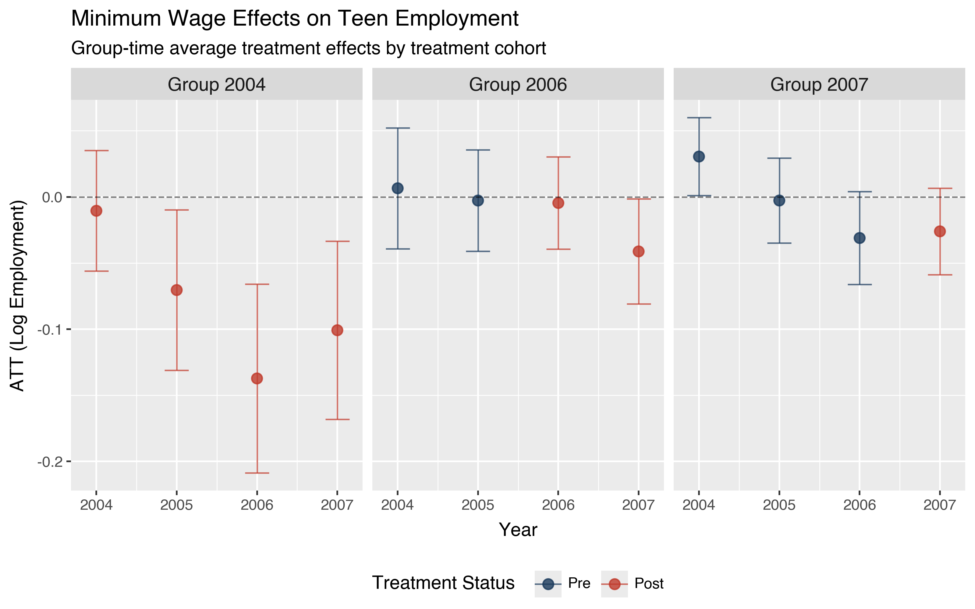
Each row represents a specific cohort (gname) measured at a specific time
(tname). Cohorts are defined by when they first received treatment. For
the 2004 cohort, the rows for 2004-2007 show how the treatment effect
evolves from the year of adoption through three years later.
Rows where Time is less than Group are pre-treatment periods. You want these to be close to zero, since large pre-treatment differences would cast doubt on the parallel trends assumption. Keep in mind that flat pre-trends are reassuring but do not guarantee parallel trends holds in the post-treatment period.
For the 2007 cohort, the estimates at times 2004, 2005, and 2006 are all pre-treatment. The estimate of 0.0305 in 2004 is slightly positive and barely significant with pointwise confidence bands, but the joint pre-test p-value of 0.1681 is the more relevant measure since we are examining multiple pre-treatment periods simultaneously. We cannot reject parallel trends at conventional levels. A low p-value here would be a warning sign that the identifying assumption may be violated.
For the 2004 cohort, effects grow from -0.01 in 2004 to -0.07 in 2005 and -0.14 in 2006 before moderating to -0.10 in 2007. This pattern of growing then partially reverting is common and suggests the policy had a lagged impact that took time to fully materialize. The 2006 and 2007 cohorts show smaller effects, possibly because they have fewer post-treatment periods for the impact to accumulate.
Aggregating into an event study#
With 12 group-time estimates, there is a lot to take in. The event study aggregation simplifies things by aligning all cohorts relative to their treatment date, making it much easier to see the overall pattern.
event_study = did.aggte(result, type="dynamic")
print(event_study)
==============================================================================
 Aggregate Treatment Effects (Event Study)
==============================================================================

 Overall summary of ATT's based on event-study/dynamic aggregation:

┌─────────┬────────────┬────────────────────────┐
│     ATT │ Std. Error │ [95% Conf. Interval]   │
├─────────┼────────────┼────────────────────────┤
│ -0.0772 │     0.0200 │ [ -0.1164,  -0.0381] * │
└─────────┴────────────┴────────────────────────┘


 Dynamic Effects:

┌────────────┬──────────┬────────────┬────────────────────────────┐
│ Event time │ Estimate │ Std. Error │ [95% Pointwise Conf. Band] │
├────────────┼──────────┼────────────┼────────────────────────────┤
│         -3 │   0.0305 │     0.0150 │ [-0.0093,  0.0703]         │
│         -2 │  -0.0006 │     0.0133 │ [-0.0357,  0.0346]         │
│         -1 │  -0.0245 │     0.0142 │ [-0.0621,  0.0132]         │
│          0 │  -0.0199 │     0.0118 │ [-0.0512,  0.0114]         │
│          1 │  -0.0510 │     0.0169 │ [-0.0957, -0.0062] *       │
│          2 │  -0.1373 │     0.0364 │ [-0.2337, -0.0408] *       │
│          3 │  -0.1008 │     0.0344 │ [-0.1918, -0.0099] *       │
└────────────┴──────────┴────────────┴────────────────────────────┘

------------------------------------------------------------------------------
 Signif. codes: '*' confidence band does not cover 0

------------------------------------------------------------------------------
 Data Info
------------------------------------------------------------------------------
 Control Group: Never Treated
 Anticipation Periods: 0

------------------------------------------------------------------------------
 Estimation Details
------------------------------------------------------------------------------
 Estimation Method: Doubly Robust

------------------------------------------------------------------------------
 Inference
------------------------------------------------------------------------------
 Significance level: 0.05
 Analytical standard errors
==============================================================================
 Reference: Callaway and Sant'Anna (2021)
Event time 0 is the year of treatment adoption. Negative event times are pre-treatment periods that serve as a placebo test for parallel trends. Positive event times show how effects evolve after treatment.
The pre-treatment estimates at event times -3, -2, and -1 are all close to zero and statistically insignificant. This is reassuring. If these were large or showed a trending pattern, it would suggest treated and control counties were already diverging before the policy change, calling into question whether the post-treatment differences reflect the policy or pre-existing trends.
The effect is small and insignificant on impact (event time 0), but we see it grow to -0.05 after one year and -0.14 after two years. This lag makes economic sense. Employers may not immediately respond to a minimum wage increase. They may first absorb higher costs, then gradually reduce hours or hiring as contracts expire and business conditions allow adjustments. The effect moderates slightly at event time 3, though this estimate is based on fewer cohorts and is less precisely estimated.
Summarizing the overall effect#
Sometimes you just need a single number to summarize the overall treatment
effect. The "simple" aggregation provides exactly that by averaging
across all post-treatment group-time cells, weighted by group size.
simple = did.aggte(result, type="simple")
print(simple)
==============================================================================
 Aggregate Treatment Effects
==============================================================================

 Overall ATT:

┌─────────┬────────────┬────────────────────────┐
│     ATT │ Std. Error │ [95% Conf. Interval]   │
├─────────┼────────────┼────────────────────────┤
│ -0.0400 │     0.0120 │ [ -0.0635,  -0.0164] * │
└─────────┴────────────┴────────────────────────┘

------------------------------------------------------------------------------
 Signif. codes: '*' confidence band does not cover 0

------------------------------------------------------------------------------
 Data Info
------------------------------------------------------------------------------
 Control Group: Never Treated
 Anticipation Periods: 0

------------------------------------------------------------------------------
 Estimation Details
------------------------------------------------------------------------------
 Estimation Method: Doubly Robust

------------------------------------------------------------------------------
 Inference
------------------------------------------------------------------------------
 Significance level: 0.05
 Analytical standard errors
==============================================================================
 Reference: Callaway and Sant'Anna (2021)
The overall ATT of -0.04 means that minimum wage increases reduced log teen employment by about 4 log points (approximately 4 percent) on average across all treated counties and post-treatment periods. The confidence interval of [-0.06, -0.02] excludes zero, indicating this effect is statistically significant.
This single number is useful for policy summaries but masks the treatment effect heterogeneity we saw in the event study. It is generally a good idea to examine the dynamic effects before reporting only the overall ATT.
Examining heterogeneity by cohort#
We might expect different cohorts to experience different effects due to
variation in local economic conditions, policy implementation, or the
composition of affected workers. The "group" aggregation reveals this
heterogeneity.
by_group = did.aggte(result, type="group")
print(by_group)
==============================================================================
 Aggregate Treatment Effects (Group/Cohort)
==============================================================================

 Overall summary of ATT's based on group/cohort aggregation:

┌─────────┬────────────┬────────────────────────┐
│     ATT │ Std. Error │ [95% Conf. Interval]   │
├─────────┼────────────┼────────────────────────┤
│ -0.0310 │     0.0124 │ [ -0.0554,  -0.0066] * │
└─────────┴────────────┴────────────────────────┘


 Group Effects:

┌───────┬──────────┬────────────┬────────────────────────────┐
│ Group │ Estimate │ Std. Error │ [95% Pointwise Conf. Band] │
├───────┼──────────┼────────────┼────────────────────────────┤
│  2004 │  -0.0797 │     0.0264 │ [-0.1378, -0.0217] *       │
│  2006 │  -0.0229 │     0.0167 │ [-0.0597,  0.0139]         │
│  2007 │  -0.0261 │     0.0167 │ [-0.0627,  0.0106]         │
└───────┴──────────┴────────────┴────────────────────────────┘

------------------------------------------------------------------------------
 Signif. codes: '*' confidence band does not cover 0

------------------------------------------------------------------------------
 Data Info
------------------------------------------------------------------------------
 Control Group: Never Treated
 Anticipation Periods: 0

------------------------------------------------------------------------------
 Estimation Details
------------------------------------------------------------------------------
 Estimation Method: Doubly Robust

------------------------------------------------------------------------------
 Inference
------------------------------------------------------------------------------
 Significance level: 0.05
 Analytical standard errors
==============================================================================
 Reference: Callaway and Sant'Anna (2021)
The 2004 cohort experienced the largest effect at -0.08, which is statistically significant. The 2006 and 2007 cohorts show effects around -0.02 to -0.03 that are not statistically significant. This heterogeneity could arise for several reasons. Early adopters may have implemented larger minimum wage increases. They also have more post-treatment periods in the data, so their effects have had more time to materialize. Or the economic conditions in 2004 may have made employment more sensitive to wage floors than in later years.
When you see this much heterogeneity across cohorts, it is worth considering whether a single overall effect tells the full story. Reporting both the event study and cohort-specific effects gives your readers a more complete picture.
Plotting results#
Visualizations make it easier to communicate findings and spot patterns. We can plot the group-time estimates organized by cohort.
from plotnine import element_text, labs, theme, theme_gray

p = did.plot_gt(result, ncol=3)
p = (p
    + labs(
        x="Year",
        y="ATT (Log Employment)",
        title="Minimum Wage Effects on Teen Employment",
        subtitle="Group-time average treatment effects by treatment cohort",
    )
    + theme_gray()
    + theme(
        legend_position="bottom",
        strip_text=element_text(size=11, weight="bold"),
    )
)
p.save("plot_gt.png", dpi=200, width=8, height=5)
The event study plot is typically the most informative visualization for staggered designs. It clearly shows both the pre-trend test and the post-treatment dynamics.
p = did.plot_event_study(event_study, ref_period=-1)
p = (p
    + labs(
        x="Years Relative to Treatment",
        y="ATT (Log Employment)",
        title="Minimum Wage Effects on Teen Employment",
        subtitle="Dynamic treatment effects from Callaway and Sant'Anna (2021)",
    )
    + theme_gray()
    + theme(legend_position="bottom")
)
p.save("plot_event_study.png", dpi=200, width=8, height=5)
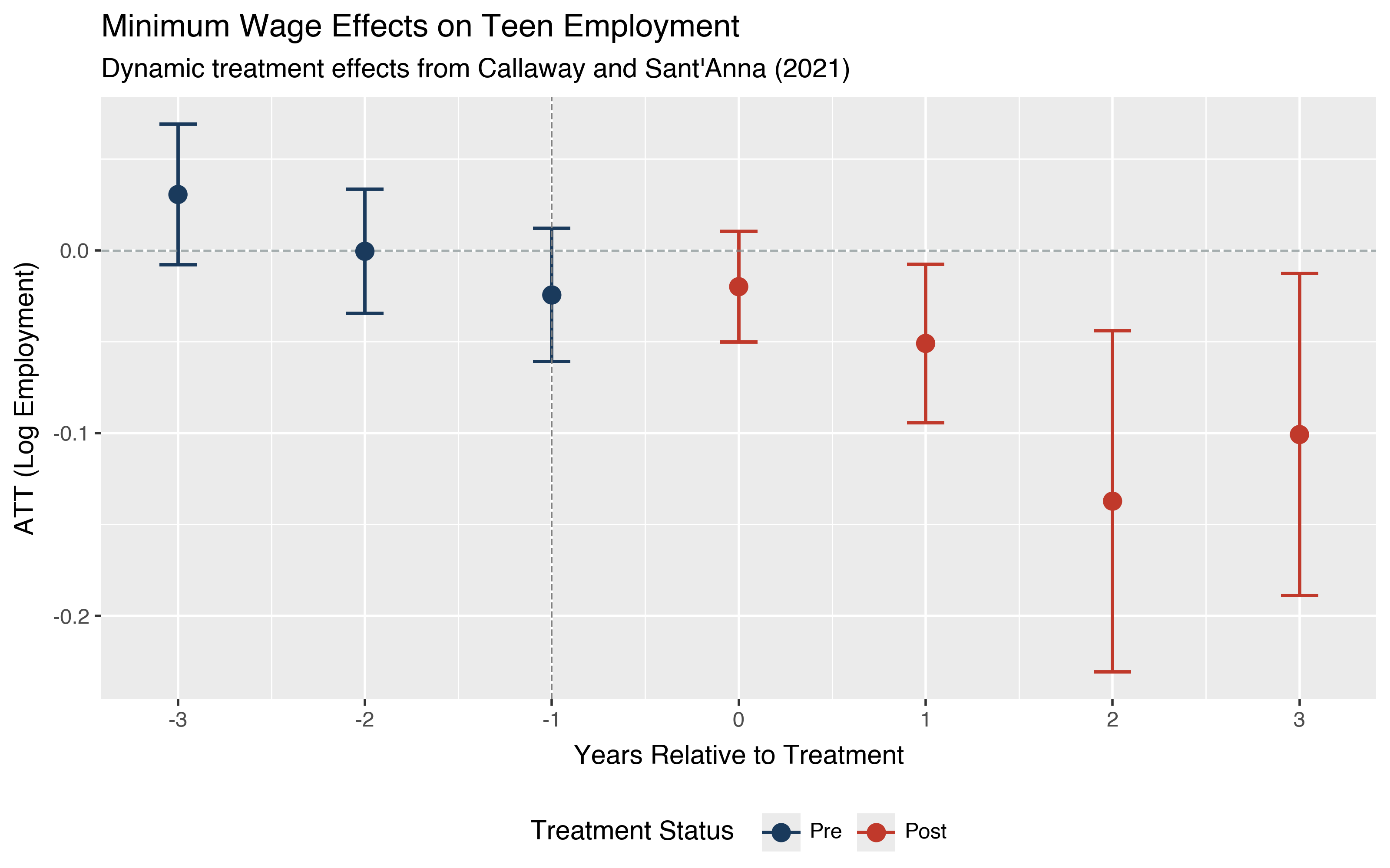
The flat pre-treatment estimates and the growing post-treatment effects tell a clear story. This is the kind of pattern that builds confidence in a causal interpretation.
Next steps#
For details on estimation options such as covariates, control groups, bootstrap inference, and clustering, see the Staggered DiD API reference.
For theoretical background on the Callaway and Sant’Anna estimator, see the Background section.
For related methods, see the Continuous DiD walkthrough for non-binary treatments and the Honest DiD sensitivity analysis for assessing robustness of these estimates to violations of parallel trends.